Julia GLM.jl and MixedModels.jl based implementation of the cluster-based permutation test for time series data, powered by JuliaConnectoR.
Installation and usage
Zero-setup test drive
As of March 2025, Google Colab supports Julia. This means jlmerclusterperm just works out of the box. Try it out in a demo notebook that runs some of the code from the Ito et al. 2018 case study vignette.
Local setup
Install the released version of jlmerclusterperm from CRAN:
install.packages("jlmerclusterperm")Or install the development version from GitHub with:
# install.packages("remotes")
remotes::install_github("yjunechoe/jlmerclusterperm")
Using jlmerclusterperm requires a prior installation of the Julia programming language, which can be downloaded from either the official website or using the command line utility juliaup. Julia version >=1.8 is required and 1.9 or higher is preferred for the substantial speed improvements.
Before using functions from jlmerclusterperm, an initial setup is required via calling jlmerclusterperm_setup(). The very first call on a system will install necessary dependencies (this only happens once and takes around 10-15 minutes).
Subsequent calls to jlmerclusterperm_setup() incur a small overhead of around 30 seconds, plus slight delays for first-time function calls. You pay up front for start-up and warm-up costs and get blazingly-fast functions from the package.
# Both lines must be run at the start of each new session
library(jlmerclusterperm)
jlmerclusterperm_setup()
See the Get Started page on the package website for background and tutorials.
Quick tour of package functionalities
Wholesale CPA with clusterpermute()
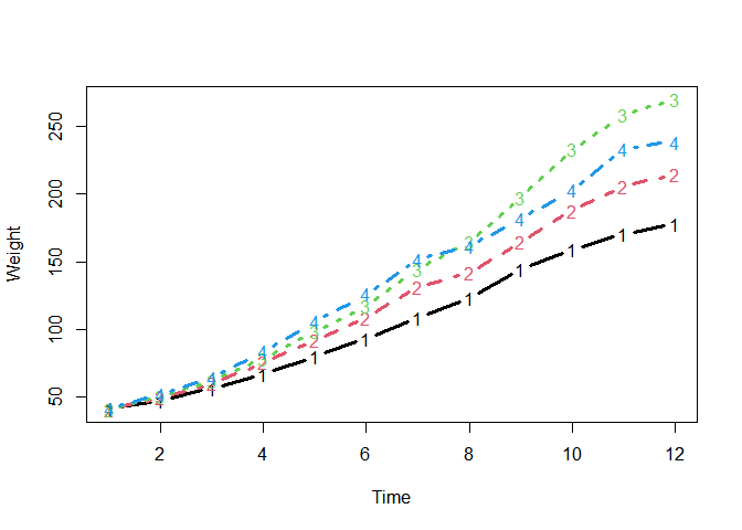
A time series data:
chickweights <- ChickWeight
chickweights$Time <- as.integer(factor(chickweights$Time))
matplot(
  tapply(chickweights$weight, chickweights[c("Time", "Diet")], mean),
  type = "b", lwd = 3, ylab = "Weight", xlab = "Time"
)
Preparing a specification object with make_jlmer_spec():
chickweights_spec <- make_jlmer_spec(
  formula = weight ~ 1 + Diet,
  data = chickweights,
  subject = "Chick", time = "Time"
)
chickweights_spec
Cluster-based permutation test with clusterpermute():
set_rng_state(123L)
clusterpermute(
  chickweights_spec,
  threshold = 2.5,
  nsim = 100
)
Including random effects:
chickweights_re_spec <- make_jlmer_spec(
  formula = weight ~ 1 + Diet + (1 | Chick),
  data = chickweights,
  subject = "Chick", time = "Time"
)
set_rng_state(123L)
clusterpermute(
  chickweights_re_spec,
  threshold = 2.5,
  nsim = 100
)$empirical_clusters
Piecemeal approach to CPA
Computing time-wise statistics of the observed data:
empirical_statistics <- compute_timewise_statistics(chickweights_spec)
matplot(t(empirical_statistics), type = "b", pch = 1, lwd = 3, ylab = "t-statistic")
abline(h = 2.5, lty = 3)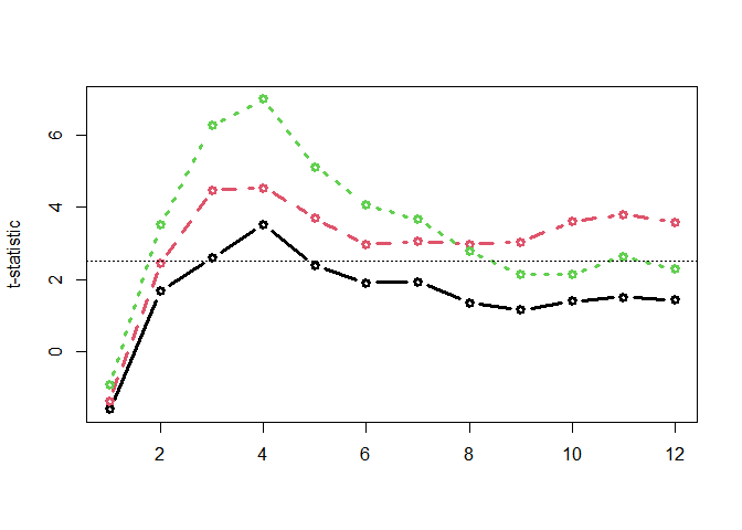
Identifying empirical clusters:
empirical_clusters <- extract_empirical_clusters(empirical_statistics, threshold = 2.5)
empirical_clusters
Simulating the null distribution:
set_rng_state(123L)
null_statistics <- permute_timewise_statistics(chickweights_spec, nsim = 100)
null_cluster_dists <- extract_null_cluster_dists(null_statistics, threshold = 2.5)
null_cluster_dists
Significance testing the cluster-mass statistic:
calculate_clusters_pvalues(empirical_clusters, null_cluster_dists, add1 = TRUE)
Iterating over a range of threshold values:
walk_threshold_steps(empirical_statistics, null_statistics, steps = c(2, 2.5, 3))
Acknowledgments
The paper Maris & Oostenveld (2007) which originally proposed the cluster-based permutation analysis.
The JuliaConnectoR package for powering the R interface to Julia.
The Julia packages GLM.jl and MixedModels.jl for fast implementations of (mixed effects) regression models.
Existing implementations of CPA in R (permuco, permutes, etc.) whose designs inspired the CPA interface in jlmerclusterperm.
Citations
If you use jlmerclusterperm for cluster-based permutation test with mixed-effects models in your research, please cite one (or more) of the following as you see fit.
To cite jlmerclusterperm:
- Choe, J. (2024). jlmerclusterperm: Cluster-Based Permutation Analysis for Densely Sampled Time Data. R package version 1.1.4. 10.32614/CRAN.package.jlmerclusterperm.
To cite the cluster-based permutation test:
- Maris, E., & Oostenveld, R. (2007). Nonparametric statistical testing of EEG- and MEG-data. Journal of Neuroscience Methods, 164, 177–190. doi: 10.1016/j.jneumeth.2007.03.024.
To cite the Julia programming language:
- Bezanson, J., Edelman, A., Karpinski, S., & Shah, V. B. (2017). Julia: A Fresh Approach to Numerical Computing. SIAM Review, 59(1), 65–98. doi: 10.1137/141000671.
To cite the GLM.jl and MixedModels.jl Julia libraries, consult their Zenodo pages: