de Carvalho et al. 2021

This tutorial is a walkthrough of contrasts for multi-level predictors (vs. multiple t-tests) and model complexity (linear vs. logistic; fixed vs. mixed) as they relate to CPA.

See more tutorials and vignettes on the Articles page.

Background

The data comes from an eye-tracking study by de Carvalho, Dautriche, Fiévet, & Christophe (2021) “Toddlers exploit referential and syntactic cues to flexibly adapt their interpretation of novel verb meanings.”

This article reproduces and expands on their Experiment 2 analysis, which used CPA (with t-tests) to conduct a pairwise comparison of the three conditions (relevant Figure 7 from the paper below).

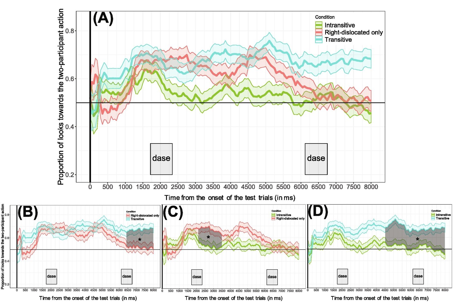
The data comes mostly ready for CPA straight from the study’s OSF repository. The collapsible chunk below contains the code to prepare the data and reproduce the figure.

Code to reproduce data and plot

Data cleaning

library(dplyr)
library(forcats)
filepath <- "https://osf.io/download/var2h/?view_only=2a06746ba360446e9857df73307d21be"
E2_data_raw <- readr::read_delim(filepath)

E2_data <- E2_data_raw %>%
  filter(away != 1) %>%
  mutate(Target = as.integer(bin_2P == 1)) %>%
  mutate(Condition = fct_recode(
    factor(Condition, levels = c("intrans", "pros", "trans")),
    "Intransitive" = "intrans",
    "RightDislocated" = "pros",
    "Transitive" = "trans"
  )) %>%
  select(Subject, Trial, Condition, Time, Target)
E2_data_agg <- E2_data %>%
  group_by(Subject, Condition, Time) %>%
  summarize(Prop = mean(Target), .groups = "drop")

# Unaggregated trial-level data of 1s and 0s
E2_data
#> # A tibble: 69,123 × 5
#>    Subject Trial Condition        Time Target
#>    <chr>   <dbl> <fct>           <dbl>  <int>
#>  1 200.asc     0 RightDislocated     0      0
#>  2 200.asc     0 RightDislocated   400      0
#>  3 200.asc     0 RightDislocated   450      1
#>  4 200.asc     0 RightDislocated   500      1
#>  5 200.asc     0 RightDislocated   550      1
#>  6 200.asc     0 RightDislocated   600      1
#>  7 200.asc     0 RightDislocated   650      1
#>  8 200.asc     0 RightDislocated   700      1
#>  9 200.asc     0 RightDislocated   750      1
#> 10 200.asc     0 RightDislocated   800      1
#> # ℹ 69,113 more rows

# Aggregated subject-mean proportions data used in original study
E2_data_agg
#> # A tibble: 11,540 × 4
#>    Subject Condition        Time  Prop
#>    <chr>   <fct>           <dbl> <dbl>
#>  1 200.asc RightDislocated     0 0.5  
#>  2 200.asc RightDislocated    50 1    
#>  3 200.asc RightDislocated   100 1    
#>  4 200.asc RightDislocated   150 1    
#>  5 200.asc RightDislocated   200 1    
#>  6 200.asc RightDislocated   250 0.5  
#>  7 200.asc RightDislocated   300 0.5  
#>  8 200.asc RightDislocated   350 0.4  
#>  9 200.asc RightDislocated   400 0.286
#> 10 200.asc RightDislocated   450 0.429
#> # ℹ 11,530 more rows

Code for Figure 7 plots

library(ggplot2)
make_fig7_plot <- function(conditions) {
  E2_data %>%
    group_by(Condition, Time) %>%
    summarize(
      Prop = mean(Target), se = sqrt(var(Target) / n()),
      lower = Prop - se, upper = Prop + se,
      .groups = "drop"
    ) %>%
    filter(Condition %in% conditions) %>%
    ggplot(aes(Time, Prop, color = Condition, fill = Condition)) +
    geom_hline(aes(yintercept = .5)) +
    geom_ribbon(
      aes(ymin = lower, ymax = upper),
      alpha = .2,
      show.legend = FALSE,
    ) +
    geom_line(linewidth = 1) +
    scale_color_manual(
      aesthetics = c("color", "fill"),
      values = setNames(scales::hue_pal()(3)[c(2, 1, 3)], levels(E2_data$Condition))
    ) +
    scale_y_continuous(limits = c(.2, .8), oob = scales::oob_keep) +
    labs(y = NULL, x = NULL) +
    theme_minimal() +
    theme(axis.title.y = element_text(angle = 0, vjust = .5, hjust = 0))
}
fig7_comparisons <- list(
  "A" = c("Intransitive", "RightDislocated", "Transitive"),
  "B" = c("RightDislocated", "Transitive"),
  "C" = c("Intransitive", "RightDislocated"),
  "D" = c("Intransitive", "Transitive")
)
fig7 <- lapply(fig7_comparisons, make_fig7_plot)

# Figure 7 combined plots
library(patchwork)
p_top <- fig7$A +
  scale_x_continuous(breaks = scales::breaks_width(1000)) +
  theme(legend.position = "bottom")
p_bot <- (fig7$B + fig7$C + fig7$D) & guides(color = guide_none())
fig7_combined <- p_top / guide_area() / p_bot +
  plot_layout(guides = "collect", heights = c(3, .1, 1)) +
  plot_annotation(tag_levels = "A")

Below is the data from the original study (as close as I could reproduce it). The E2_data_agg dataframe has the following four columns:

• Subject: Unique identifier for subjects
• Condition: A between-participant factor variable with three levels ("Intransitive", "RightDislocated", "Transitive")
• Time: A continuous measure of time from 0-8000ms in 50ms intervals
• Prop: Proportion of looks to the target (averaged across trials within each condition, by subject)

E2_data_agg
#> # A tibble: 11,540 × 4
#>    Subject Condition        Time  Prop
#>    <chr>   <fct>           <dbl> <dbl>
#>  1 200.asc RightDislocated     0 0.5  
#>  2 200.asc RightDislocated    50 1    
#>  3 200.asc RightDislocated   100 1    
#>  4 200.asc RightDislocated   150 1    
#>  5 200.asc RightDislocated   200 1    
#>  6 200.asc RightDislocated   250 0.5  
#>  7 200.asc RightDislocated   300 0.5  
#>  8 200.asc RightDislocated   350 0.4  
#>  9 200.asc RightDislocated   400 0.286
#> 10 200.asc RightDislocated   450 0.429
#> # ℹ 11,530 more rows

The following is a reproduction of Figure 7 from the original paper:

fig7_combined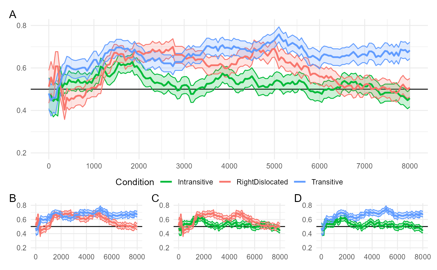

The original study used pairwise comparisons to analyze the relationship between the three conditions. The smaller figures (B, C, D) plot the following relationships:

• (B) More looks to the target in "Transitive" compared to "RightDislocated"
• (C) More looks to the target in "RightDislocated" compared to "Intransitive"
• (D) More looks to the target in "Transitive" compared to "Intransitive"

The rest of this vignette is organized as follows:

• First, we replicate the individual pairwise CPAs from the original paper.

• Next, we consider a more parsimonious analysis that reformulates the same research hypothesis as a choice of regression contrast.

• Lastly, we build on the model from (2) and consider issues around model diagnostics and complexity (linear vs. logistic; fixed vs. mixed) in the context of CPA

Load the package and start the Julia instance with jlmerclusterperm_setup() before proceeding.

library(jlmerclusterperm)
jlmerclusterperm_setup(verbose = FALSE)

Replicating the pairwise CPAs

The three conditions in the experiment are levels of the Condition factor variable:

levels(E2_data_agg$Condition)
#> [1] "Intransitive"    "RightDislocated" "Transitive"

We begin with a replication of the "Transitive" vs. "RightDislocated" comparison shown in Figure 7B and apply the same logic to the other two pairwise comparisons in 7C and 7D.

Transitive vs. RightDislocated

The reproduced Figure 7B below compares "Transitive" and "RightDislocated" conditions.

fig7$B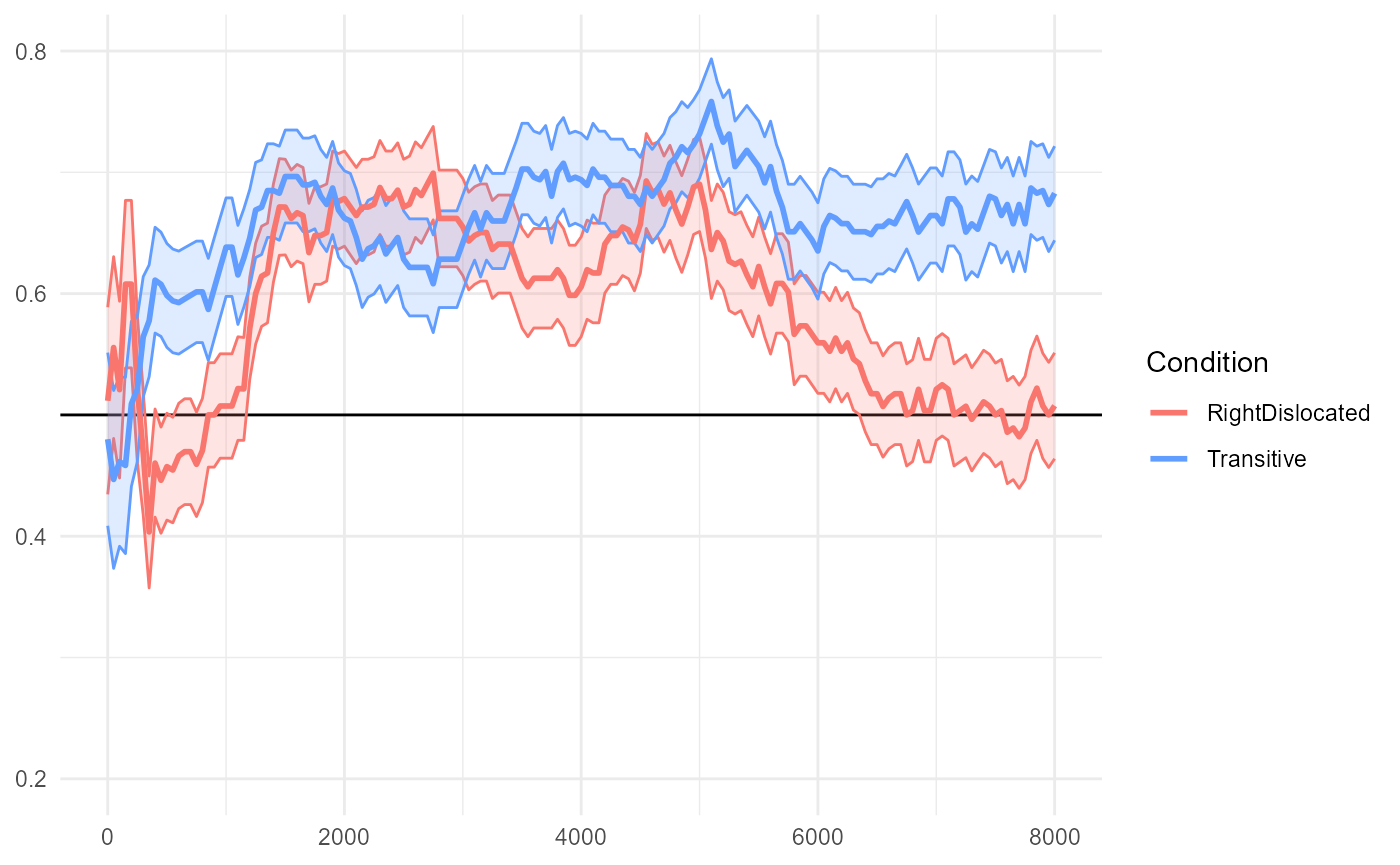

The paper (in the caption for Figure 7; emphasis mine) reports:

The transitive and right-dislocated conditions differed from each other from the second repetition of the novel verbs (~6400 ms after the onset of the test trials until the end of the trials).

We now replicate this analysis.

First, we prepare a specification object. Two things to note here:

• We express the original t-test as a regression model with Condition as the predictor
• We drop the third, unused condition from the data and from the factor representation

spec_7B <- make_jlmer_spec(
  formula = Prop ~ Condition,
  data = E2_data_agg %>%
    filter(Condition %in% c("Transitive", "RightDislocated")) %>%
    mutate(Condition = droplevels(Condition)), # or forcats::fct_drop()
  subject = "Subject", time = "Time"
)
spec_7B
#> ── jlmer specification ───────────────────────────────────────── <jlmer_spec> ──
#> Formula: Prop ~ 1 + ConditionTransitive
#> Predictors:
#>   Condition: ConditionTransitive
#> Groupings:
#>   Subject: Subject
#>   Trial:
#>   Time: Time
#> Data:
#> # A tibble: 7,688 × 4
#>    Prop ConditionTransitive Subject  Time
#>   <dbl>               <dbl> <chr>   <dbl>
#> 1   0.5                   0 200.asc     0
#> 2   1                     0 200.asc    50
#> 3   1                     0 200.asc   100
#> # ℹ 7,685 more rows
#> ────────────────────────────────────────────────────────────────────────────────

Next, we fit a global model to sanity check the structure of the model output. We get one estimate for ConditionTransitive which has a positive coefficient, as we’d expect:

jlmer(spec_7B)
#> <Julia object of type StatsModels.TableRegressionModel>
#> ──────────────────────────────────────────────────────────────────────────────────
#>                          Coef.  Std. Error       z  Pr(>|z|)  Lower 95%  Upper 95%
#> ──────────────────────────────────────────────────────────────────────────────────
#> (Intercept)          0.592999   0.00364424  162.72    <1e-99   0.585856  0.600141
#> ConditionTransitive  0.0569017  0.0051591    11.03    <1e-27   0.04679   0.0670133
#> ──────────────────────────────────────────────────────────────────────────────────

Finally, we call clusterpermute() with threshold = 1.5 (same as in the original study) and simulate 100 permutations:

clusterpermute(spec_7B, threshold = 1.5, nsim = 100L, progress = FALSE)
#> $null_cluster_dists
#> ── Null cluster-mass distribution (t > 1.5) ──────────── <null_cluster_dists> ──
#> ConditionTransitive (n = 100)
#>   Mean (SD): -2.674 (27.83)
#>   Coverage intervals: 95% [-61.740, 46.439]
#> ────────────────────────────────────────────────────────────────────────────────
#> 
#> $empirical_clusters
#> ── Empirical clusters (t > 1.5) ──────────────────────── <empirical_clusters> ──
#> ConditionTransitive
#>   [300, 1150]: 40.643 (p=0.1287)
#>   [2700, 2750]: -4.068 (p=0.9010)
#>   [6150, 6200]: 3.249 (p=0.9505)
#>   [6400, 8000]: 88.742 (p=0.0198)
#> ────────────────────────────────────────────────────────────────────────────────

We detect the same largest empirical cluster spanning 6400-8000ms as reported in the original paper. This converges to around p=0.02 in a separate 10,000-simulation run (not shown here).

RightDislocated vs. Intransitive

The reproduced Figure 7C below compares "RightDislocated" and "Intransitive" conditions.

fig7$C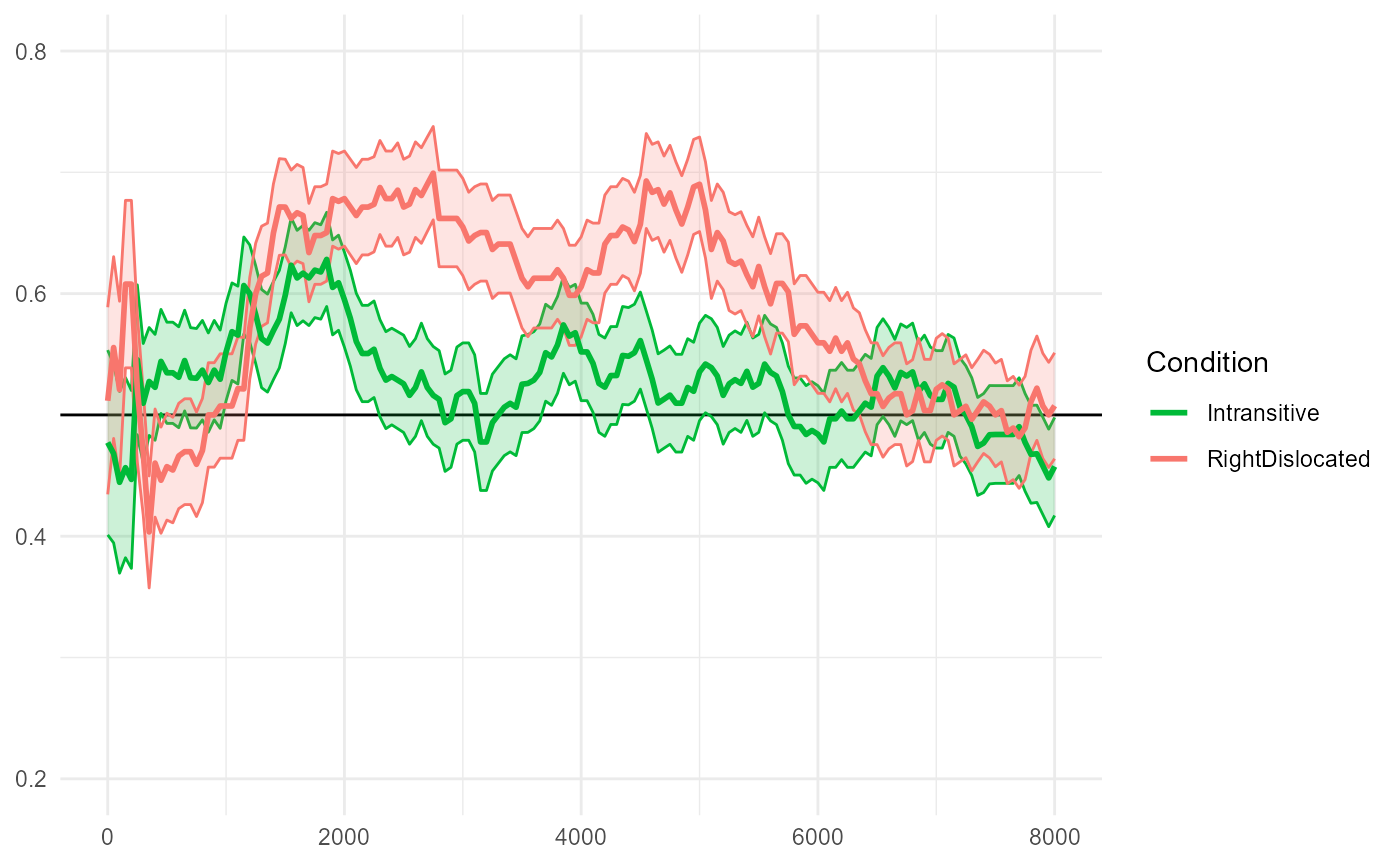

The paper reports:

The intransitive and right-dislocated conditions differed from each other from the first repetition of the novel verbs (from 2100 ms until 3500 ms after the beginning of the test trials).

We repeat the same CPA procedure for this pairwise comparison:

spec_7C <- make_jlmer_spec(
  formula = Prop ~ Condition,
  data = E2_data_agg %>%
    filter(Condition %in% c("RightDislocated", "Intransitive")) %>%
    mutate(Condition = droplevels(Condition)),
  subject = "Subject", time = "Time"
)

clusterpermute(spec_7C, threshold = 1.5, nsim = 100L, progress = FALSE)
#> $null_cluster_dists
#> ── Null cluster-mass distribution (t > 1.5) ──────────── <null_cluster_dists> ──
#> ConditionRightDislocated (n = 100)
#>   Mean (SD): 0.619 (33.26)
#>   Coverage intervals: 95% [-63.734, 67.326]
#> ────────────────────────────────────────────────────────────────────────────────
#> 
#> $empirical_clusters
#> ── Empirical clusters (t > 1.5) ──────────────────────── <empirical_clusters> ──
#> ConditionRightDislocated
#>   [150, 200]: 3.562 (p=0.9010)
#>   [2150, 3650]: 72.842 (p=0.0297)
#>   [4550, 5050]: 23.836 (p=0.3960)
#>   [5150, 5350]: 8.589 (p=0.7723)
#>   [5700, 5750]: 3.332 (p=0.9208)
#> ────────────────────────────────────────────────────────────────────────────────

The largest empirical cluster we detect spans 2150-3650ms, which is slightly different from the cluster reported in the original paper (2100-3500ms). This is a relatively less “extreme” cluster that converges to around p=0.05 in a 10,000-simulation run.

Transitive vs. Intransitive

The reproduced Figure 7D below compares "Transitive" and "Intransitive" conditions.

fig7$D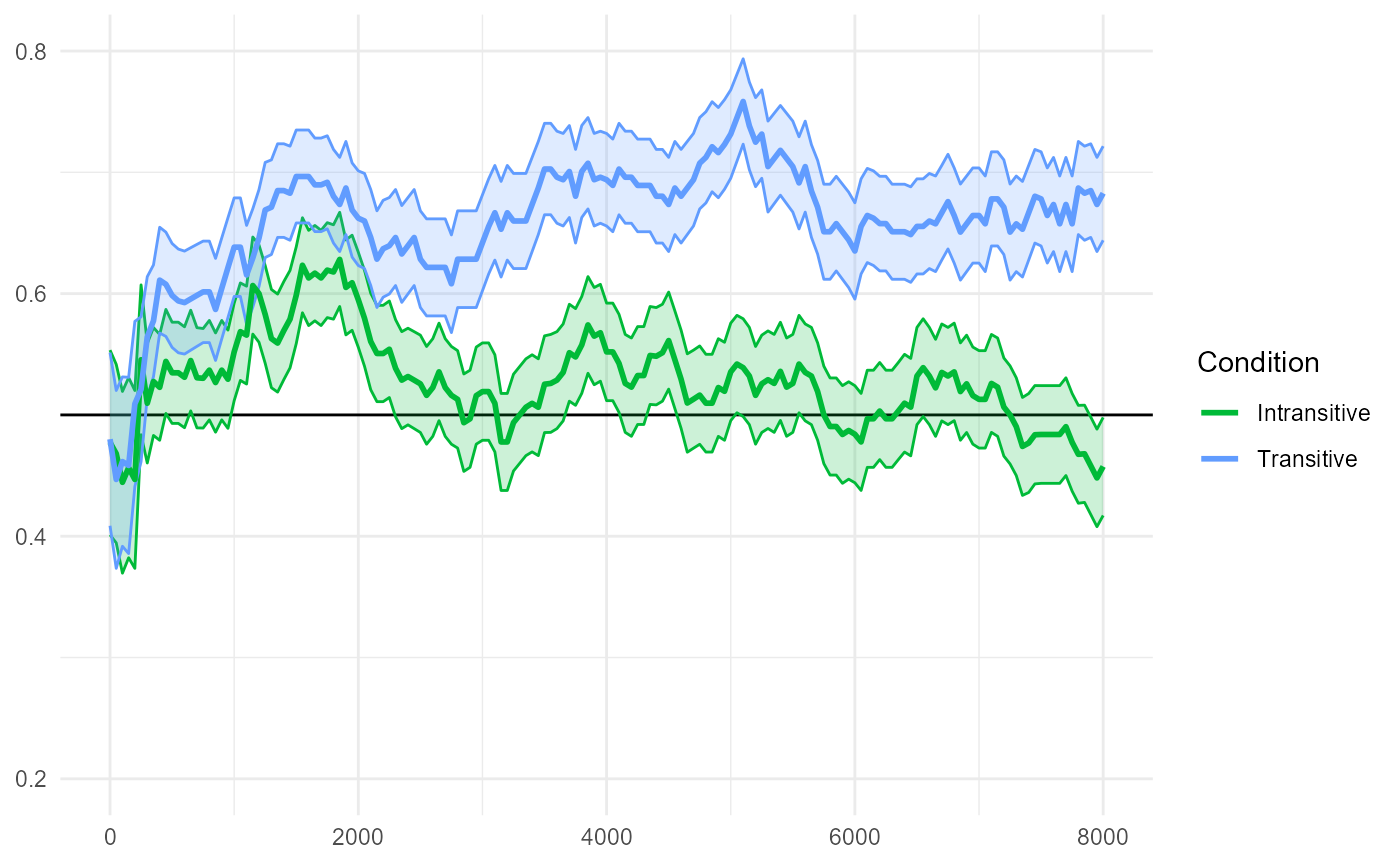

The paper reports:

The transitive and intransitive conditions differed from each other slightly after the offset of the first sentence in the test trials (from 4500 ms after the beginning of the test trials until the end of the trials).

We repeat the same CPA procedure for this pairwise comparison:

spec_7D <- make_jlmer_spec(
  formula = Prop ~ Condition,
  data = E2_data_agg %>%
    filter(Condition %in% c("Transitive", "Intransitive")) %>%
    mutate(Condition = droplevels(Condition)),
  subject = "Subject", time = "Time"
)

clusterpermute(spec_7D, threshold = 1.5, nsim = 100L, progress = FALSE)
#> $null_cluster_dists
#> ── Null cluster-mass distribution (t > 1.5) ──────────── <null_cluster_dists> ──
#> ConditionTransitive (n = 100)
#>   Mean (SD): 2.024 (41.73)
#>   Coverage intervals: 95% [-70.510, 88.501]
#> ────────────────────────────────────────────────────────────────────────────────
#> 
#> $empirical_clusters
#> ── Empirical clusters (t > 1.5) ──────────────────────── <empirical_clusters> ──
#> ConditionTransitive
#>   [300, 1000]: 25.928 (p=0.4356)
#>   [1300, 1400]: 4.808 (p=0.8713)
#>   [2800, 2900]: 5.356 (p=0.8218)
#>   [3000, 4300]: 52.638 (p=0.2079)
#>   [4600, 8000]: 172.635 (p=0.0198)
#> ────────────────────────────────────────────────────────────────────────────────

The largest empirical cluster we detect spans 4600-8000ms, which is again only slightly different from the cluster reported in the original paper (4500-8000ms). This converges to around p=0.001 in a separate 10,000-simulation run.

Expressed as regression contrasts

We now consider a more parsimonious analysis that translates the research hypothesis into contrast coding to avoid multiple testing. Specifically, we exploit the fact that the original paper only specifies the hypothesis up to Intransitive < RightDislocated < Transitive.

Helmert (deviation) coding

Testing for such an ordinal relationship between levels of a category does not require all possible pairwise comparisons; instead, it can be approximated via Helmert coding (a.k.a. deviance coding) where K levels are expressed K-1 contrasts, with each contrast successively comparing a level vs. the average of previous (typically lower) levels. Critically, because Helmert contrasts are orthogonal, we can test for them simultaneously in a single model.

For our data, we test the ordinal relationship Intransitive < RightDislocated < Transitive via these two contrasts:

1. "RightDislocated" vs. "Intransitive"
2. "Transitive" vs. the average of "RightDislocated" and "Intransitive"

The corresponding numerical coding is the following:

condition_helm <- contr.helmert(3)
colnames(condition_helm) <- c("RvsI", "TvsRI")
condition_helm
#>   RvsI TvsRI
#> 1   -1    -1
#> 2    1    -1
#> 3    0     2

In practice, Helmert contrasts are often standardized such that all deviations are expressed as a unit of 1. We also do this here such that the comparison between "RightDislocated" vs. "Intransitive" is expressed as 1 unit of RvsI and the comparison between "Transitive" vs. the average of "RightDislocated" and "Intransitive" is expressed as 1 unit of TvsRI:

condition_helm[, 1] <- condition_helm[, 1] / 2
condition_helm[, 2] <- condition_helm[, 2] / 3
condition_helm
#>   RvsI      TvsRI
#> 1 -0.5 -0.3333333
#> 2  0.5 -0.3333333
#> 3  0.0  0.6666667

Once we have our contrast matrix, we make a new column in our original data called ConditionHelm copying the Condition column, and apply the contrasts to this new column:

E2_data_agg$ConditionHelm <- E2_data_agg$Condition
contrasts(E2_data_agg$ConditionHelm) <- condition_helm

# For pretty-printing as fractions
MASS::fractions(contrasts(E2_data_agg$ConditionHelm))
#>                 RvsI TvsRI
#> Intransitive    -1/2 -1/3 
#> RightDislocated  1/2 -1/3 
#> Transitive         0  2/3

Lastly, we build a new specification making use of the full data. Here, we predict Prop with ConditionHelm which will estimate the effect of both contrasts in a single model.

spec_helm <- make_jlmer_spec(
  formula = Prop ~ ConditionHelm,
  data = E2_data_agg,
  subject = "Subject", time = "Time"
)
spec_helm
#> ── jlmer specification ───────────────────────────────────────── <jlmer_spec> ──
#> Formula: Prop ~ 1 + ConditionHelmRvsI + ConditionHelmTvsRI
#> Predictors:
#>   ConditionHelm: ConditionHelmRvsI, ConditionHelmTvsRI
#> Groupings:
#>   Subject: Subject
#>   Trial:
#>   Time: Time
#> Data:
#> # A tibble: 11,540 × 5
#>    Prop ConditionHelmRvsI ConditionHelmTvsRI Subject  Time
#>   <dbl>             <dbl>              <dbl> <chr>   <dbl>
#> 1   0.5               0.5             -0.333 200.asc     0
#> 2   1                 0.5             -0.333 200.asc    50
#> 3   1                 0.5             -0.333 200.asc   100
#> # ℹ 11,537 more rows
#> ────────────────────────────────────────────────────────────────────────────────

As a sanity check, we fit a global model - we expect an estimate for each contrast and we indeed find both RvsI and TvsRI in the output with positive coefficients. This suggests that the ordinal relationship between the three conditions hold at least globally.

jlmer(spec_helm) %>%
  tidy(effects = "fixed")
#> # A tibble: 3 × 5
#>   term               estimate std.error statistic  p.value
#>   <chr>                 <dbl>     <dbl>     <dbl>    <dbl>
#> 1 (Intercept)          0.591    0.00215     275.  0       
#> 2 ConditionHelmRvsI    0.0640   0.00526      12.2 5.67e-34
#> 3 ConditionHelmTvsRI   0.0889   0.00457      19.5 2.02e-84

Note how the coefficient for the RvsI contrast is exactly the same as that from the pairwise model using spec_7C from earlier, which also compared "RightDislocated" to "Intransitive":

jlmer(spec_7C) %>%
  tidy(effects = "fixed")
#> # A tibble: 2 × 5
#>   term                     estimate std.error statistic  p.value
#>   <chr>                       <dbl>     <dbl>     <dbl>    <dbl>
#> 1 (Intercept)                0.529    0.00379     140.  0       
#> 2 ConditionRightDislocated   0.0640   0.00536      11.9 8.30e-33

In spec_helm the two conditions in RvsI were coded as -0.5 and 0.5, and in spec_7C’s treatment coding they were coded as 0 and 1. Since both express the difference from "Intransitive" to "RightDislocated" as a unit of +1, the two coefficients are equal in magnitude and sign.

Interpreting CPA results

We proceed as normal and clusterpermute() using the new spec_helm:

reset_rng_state()
CPA_helm <- clusterpermute(spec_helm, threshold = 1.5, nsim = 100L, progress = FALSE)
CPA_helm
#> $null_cluster_dists
#> ── Null cluster-mass distribution (t > 1.5) ──────────── <null_cluster_dists> ──
#> ConditionHelmRvsI (n = 100)
#>   Mean (SD): 4.019 (28.80)
#>   Coverage intervals: 95% [-45.805, 67.827]
#> ConditionHelmTvsRI (n = 100)
#>   Mean (SD): 1.213 (24.59)
#>   Coverage intervals: 95% [-50.218, 47.462]
#> ────────────────────────────────────────────────────────────────────────────────
#> 
#> $empirical_clusters
#> ── Empirical clusters (t > 1.5) ──────────────────────── <empirical_clusters> ──
#> ConditionHelmRvsI
#>   [150, 200]: 3.654 (p=0.8911)
#>   [2150, 3650]: 71.141 (p=0.0297)
#>   [4550, 5350]: 36.043 (p=0.2079)
#>   [5700, 5750]: 3.328 (p=0.9010)
#> ConditionHelmTvsRI
#>   [300, 1050]: 35.863 (p=0.1881)
#>   [3500, 3700]: 8.348 (p=0.6436)
#>   [3850, 4250]: 15.985 (p=0.4455)
#>   [4800, 5600]: 36.143 (p=0.1782)
#>   [5800, 8000]: 123.631 (p=0.0099)
#> ────────────────────────────────────────────────────────────────────────────────

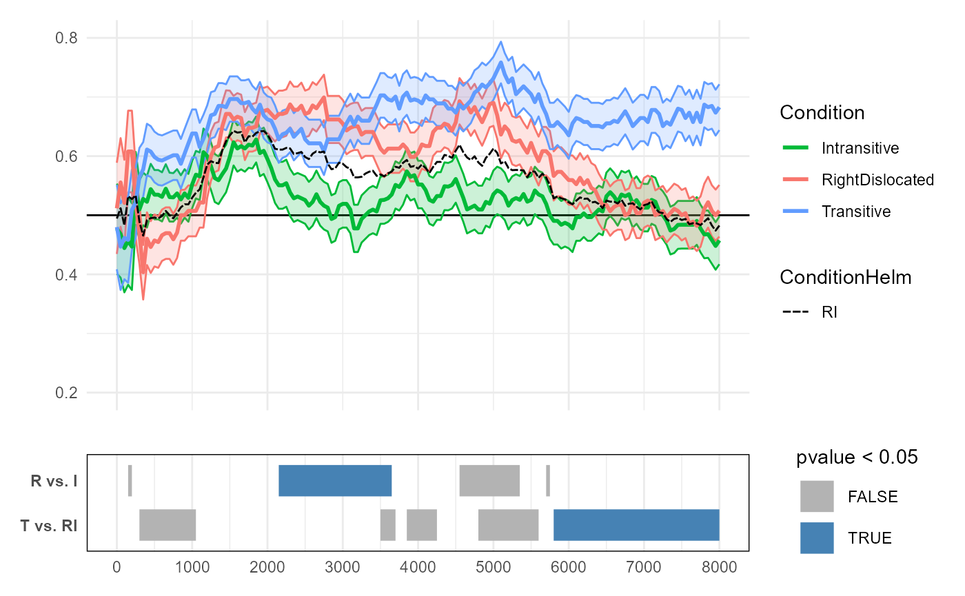
Here’s a summary of what we find from CPA_helm:

• The RvsI clusters are similar to what we detected from our previous “partial” CPA with spec_7C. The slight differences in the cluster-mass are due in part due to the Helmert-coded model simultaneously estimating the TvsRI contrast. But importantly, CPA_helm detects the same largest cluster between "RightDislocated" and "Intransitive" (2150-3650ms). This again converges to around p=0.05 in a 10,000-simulation run.

• The TvsRI clusters are new, and the largest cluster for this predictor spans 5800ms-8000ms. This converges to around p=0.01 in a separate 10,000-simulation run. This cluster effectively captures the region where the relationship Transitive > (RightDislocated & Intransitive) emerges as robust. Essentially, TvsRI is a comparison between the line for "Transitive" and an invisible line that runs in between the lines for "Intransitive" and "RightDislocated".

We conclude by visualizing the clusters for the two Helmert-coded terms, annotated below the empirical data. The “invisible” line for RI from Helmert coding is drawn as a dashed line.

Plotting code

fig7A_v2 <- fig7$A +
  geom_line(
    aes(Time, Prop, linetype = "RI"),
    inherit.aes = FALSE,
    data = . %>%
      filter(Condition %in% c("RightDislocated", "Intransitive")) %>%
      group_by(Time) %>%
      summarize(Prop = mean(Prop)),
  ) +
  scale_linetype_manual(values = "41", guide = guide_legend("ConditionHelm")) +
  guides(x = guide_none(""))

clusters_annotation <- tidy(CPA_helm$empirical_clusters) %>%
  mutate(contrast = gsub(".*([TR])vs([RI]+)", "\\1 vs. \\2", predictor)) %>%
  ggplot(aes(y = fct_rev(contrast))) +
  geom_segment(
    aes(
      x = start, xend = end, yend = contrast,
      color = pvalue < 0.05
    ),
    linewidth = 8
  ) +
  scale_color_manual(values = c("grey70", "steelblue")) +
  scale_y_discrete() +
  scale_x_continuous(n.breaks = 9, limits = range(E2_data_agg$Time)) +
  theme_minimal() +
  theme(
    axis.title = element_blank(),
    axis.text.y = element_text(face = "bold"),
    panel.border = element_rect(fill = NA),
    panel.grid.major.y = element_blank()
  )

fig7A_v2 / clusters_annotation +
  plot_layout(heights = c(4, 1))

Model complexity

We wrap up this case study by considering a more complex CPA which uses logistic mixed effects models over trial-level data of fixations to the target (1s and 0s).

Logistic mixed model

The un-aggregated trial-level data that we will use in this section is E2_data, which comes from the initial data preparation code chunk:

E2_data
#> # A tibble: 69,123 × 5
#>    Subject Trial Condition        Time Target
#>    <chr>   <dbl> <fct>           <dbl>  <int>
#>  1 200.asc     0 RightDislocated     0      0
#>  2 200.asc     0 RightDislocated   400      0
#>  3 200.asc     0 RightDislocated   450      1
#>  4 200.asc     0 RightDislocated   500      1
#>  5 200.asc     0 RightDislocated   550      1
#>  6 200.asc     0 RightDislocated   600      1
#>  7 200.asc     0 RightDislocated   650      1
#>  8 200.asc     0 RightDislocated   700      1
#>  9 200.asc     0 RightDislocated   750      1
#> 10 200.asc     0 RightDislocated   800      1
#> # ℹ 69,113 more rows

We again apply the same Helmert/deviation-coded contrast matrix:

E2_data$ConditionHelm <- E2_data$Condition
contrasts(E2_data$ConditionHelm) <- condition_helm
MASS::fractions(contrasts(E2_data$ConditionHelm))
#>                 RvsI TvsRI
#> Intransitive    -1/2 -1/3 
#> RightDislocated  1/2 -1/3 
#> Transitive         0  2/3

In our specification object for E2_data, we add trial = "Trial" and predict Target instead of Prop. We also add a by-subject random intercept to the formula:

spec_helm_complex <- make_jlmer_spec(
  formula = Target ~ ConditionHelm + (1 | Subject),
  data = E2_data,
  subject = "Subject", trial = "Trial", time = "Time"
)
spec_helm_complex
#> ── jlmer specification ───────────────────────────────────────── <jlmer_spec> ──
#> Formula: Target ~ 1 + ConditionHelmRvsI + ConditionHelmTvsRI + (1 | Subject)
#> Predictors:
#>   ConditionHelm: ConditionHelmRvsI, ConditionHelmTvsRI
#> Groupings:
#>   Subject: Subject
#>   Trial: Trial
#>   Time: Time
#> Data:
#> # A tibble: 69,123 × 6
#>   Target ConditionHelmRvsI ConditionHelmTvsRI Subject Trial  Time
#>    <int>             <dbl>              <dbl> <chr>   <dbl> <dbl>
#> 1      0               0.5             -0.333 200.asc     0     0
#> 2      0               0.5             -0.333 200.asc     0   400
#> 3      1               0.5             -0.333 200.asc     0   450
#> # ℹ 69,120 more rows
#> ────────────────────────────────────────────────────────────────────────────────

Then, we CPA with family = "binomial":

reset_rng_state()
CPA_helm_complex <- clusterpermute(
  spec_helm_complex,
  family = "binomial",
  threshold = 1.5, nsim = 100,
  progress = FALSE
)
CPA_helm_complex
#> $null_cluster_dists
#> ── Null cluster-mass distribution (t > 1.5) ──────────── <null_cluster_dists> ──
#> ConditionHelmRvsI (n = 100)
#>   Mean (SD): 1.791 (31.12)
#>   Coverage intervals: 95% [-60.956, 80.602]
#> ConditionHelmTvsRI (n = 100)
#>   Mean (SD): 2.704 (28.90)
#>   Coverage intervals: 95% [-54.636, 62.925]
#> ────────────────────────────────────────────────────────────────────────────────
#> 
#> $empirical_clusters
#> ── Empirical clusters (t > 1.5) ──────────────────────── <empirical_clusters> ──
#> ConditionHelmRvsI
#>   [2100, 3450]: 69.563 (p=0.0495)
#>   [4200, 5050]: 40.460 (p=0.1584)
#>   [5150, 5350]: 8.379 (p=0.7228)
#> ConditionHelmTvsRI
#>   [350, 800]: 19.358 (p=0.4158)
#>   [900, 1050]: 7.519 (p=0.6535)
#>   [1250, 1350]: 4.980 (p=0.7228)
#>   [3100, 4450]: 56.770 (p=0.0792)
#>   [4650, 8000]: 181.165 (p=0.0099)
#> ────────────────────────────────────────────────────────────────────────────────

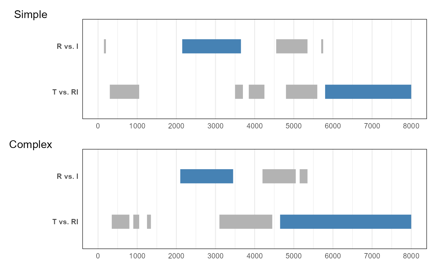
We now visualize the results of CPA_helm_complex and CPA_helm side by side:

Plotting code

clusters_annotation2 <- tidy(CPA_helm_complex$empirical_clusters) %>%
  mutate(contrast = gsub(".*([TR])vs([RI]+)", "\\1 vs. \\2", predictor)) %>%
  ggplot(aes(y = fct_rev(contrast))) +
  geom_segment(
    aes(
      x = start, xend = end, yend = contrast,
      color = pvalue < 0.05
    ),
    linewidth = 8
  ) +
  scale_color_manual(values = c("grey70", "steelblue")) +
  scale_y_discrete() +
  scale_x_continuous(n.breaks = 9, limits = range(E2_data$Time)) +
  theme_minimal() +
  theme(
    legend.position = "bottom",
    axis.title = element_blank(),
    axis.text.y = element_text(face = "bold"),
    panel.border = element_rect(fill = NA),
    panel.grid.major.y = element_blank()
  )

clusters_annotation / clusters_annotation2 &
  guides(color = guide_none()) &
  plot_annotation(tag_levels = list(c("Simple", "Complex")))

The results are largely the same, except that the largest, significant cluster identified for TvsRI extends much further in the complex CPA than the simple CPA. We examine this difference next.

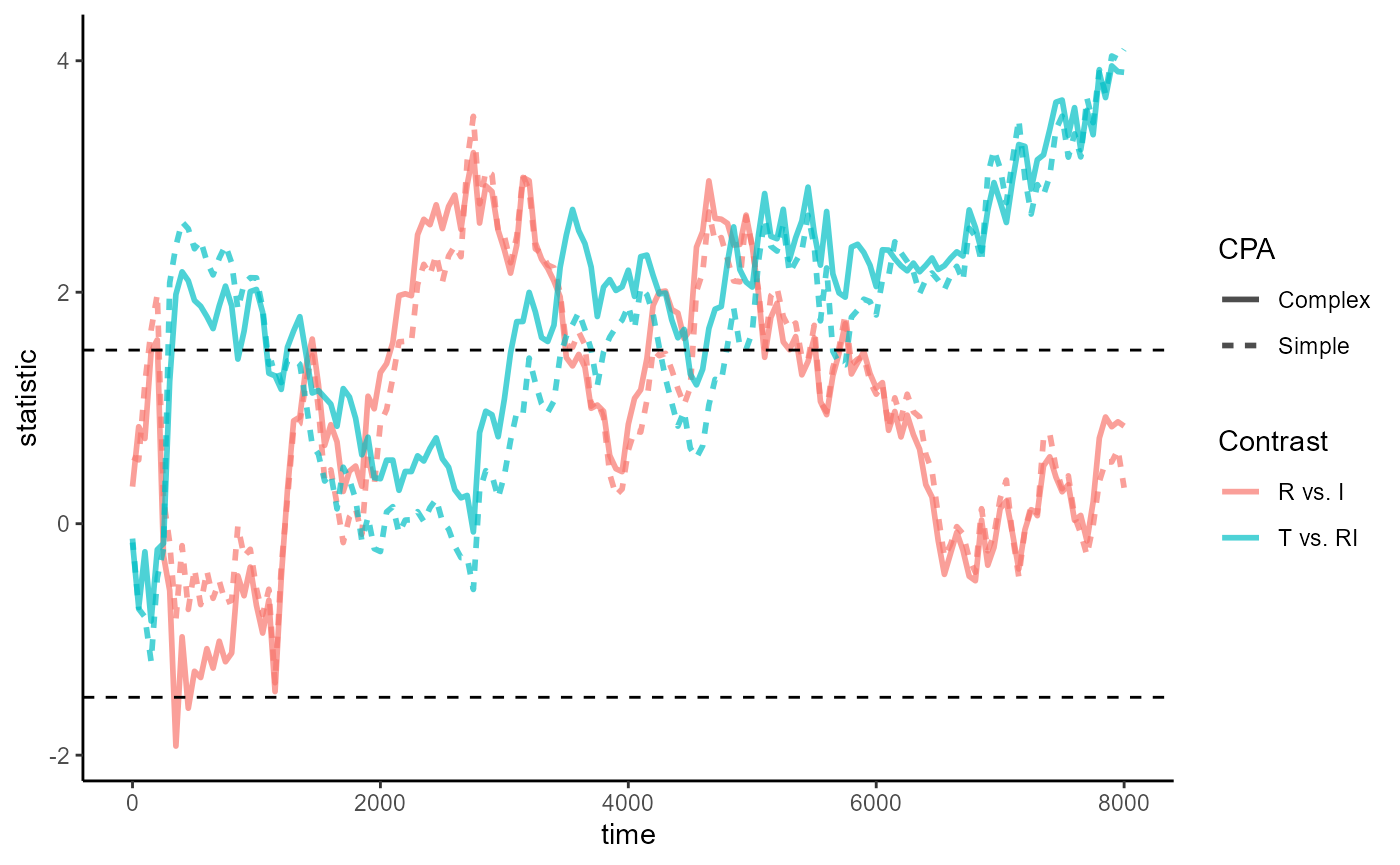
Comparison of CPAs

Looking at the timewise statistics computed in the simple vs. complex CPA tells us why. The figure below plots this information from calls to compute_timewise_statistics():

Plotting code

# Compute the timewise statistics from the CPA specifications
empirical_statistics <- bind_rows(
  tidy(compute_timewise_statistics(spec_helm)),
  tidy(compute_timewise_statistics(spec_helm_complex, family = "binomial")),
  .id = "spec"
) %>%
  mutate(
    CPA = c("Simple", "Complex")[as.integer(spec)],
    Contrast = gsub(".*([TR])vs([RI]+)", "\\1 vs. \\2", predictor)
  )

# Time series plot of the statistics, with a line for each Helmert contrasts
empirical_statistics_fig <- ggplot(empirical_statistics, aes(time, statistic)) +
  geom_line(aes(color = Contrast, linetype = CPA), linewidth = 1, alpha = .7) +
  geom_hline(yintercept = c(-1.5, 1.5), linetype = 2) +
  theme_classic()

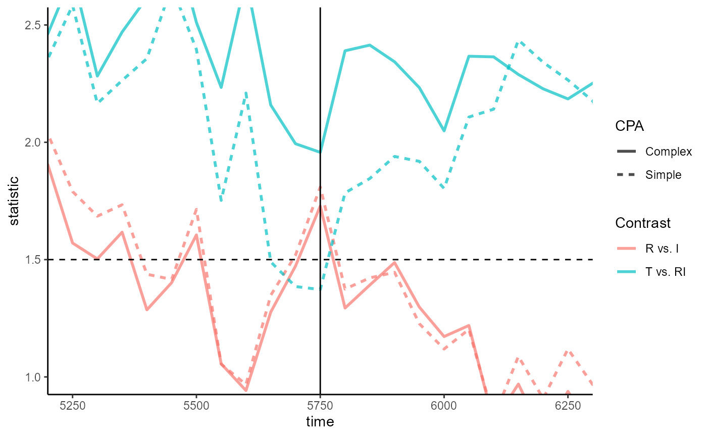
empirical_statistics_fig

Whereas the largest cluster starts to emerge at 5800ms for CPA_helm, it emerges much earlier at 4650ms for CPA_helm_complex. When we zoom into the region around 5800ms, we see that timewise statistics for T vs. RI in CPA_helm suddenly dip below the 1.5 threshold at 5750ms:

Plotting code

empirical_statistics_fig +
  geom_vline(xintercept = 5750) +
  coord_cartesian(xlim = 5750 + c(-500, 500), ylim = c(1, 2.5))

So which CPA is better? The existence of dips and spikes does not itself indicate a problem, but it’s consistent with the expectation that the simple CPA would be less robust to variance.

We can inspect the time-point model at 5750ms from the two CPAs by fitting it ourselves:

jlmer_simple_5750 <- to_jlmer(
  formula = Prop ~ ConditionHelm,
  data = E2_data_agg %>% filter(Time == 5750)
)
jlmer_complex_5750 <- to_jlmer(
  formula = Target ~ ConditionHelm + (1 | Subject),
  family = "binomial",
  data = E2_data %>% filter(Time == 5750)
)

There’s no standard way of comparing goodness of fit between a linear fixed-effects model and a logistic mixed-effects model fitted to different data. But the complex model outperforms the simple model on all the classic metrics when we inspect with glance(). This doesn’t come as a surprise, as the differences are largely driven by the number of observations (nobs).

glance(jlmer_simple_5750)
#> # A tibble: 1 × 8
#>    nobs    df sigma logLik   AIC   BIC deviance df.residual
#>   <dbl> <int> <dbl>  <dbl> <dbl> <dbl>    <dbl>       <dbl>
#> 1    72     4 0.223   7.51 -7.02  2.08     3.42          68
glance(jlmer_complex_5750)
#> # A tibble: 1 × 8
#>    nobs    df sigma logLik   AIC   BIC deviance df.residual
#>   <int> <int> <lgl>  <dbl> <dbl> <dbl>    <dbl>       <int>
#> 1   448     4 NA     -301.  609.  626.     601.         444

Determining the appropriate degree of model complexity in a CPA is beyond the scope of this vignette, so we will not pursue this discussion further. Instead, we conclude with an old wisdom: a chain is only as strong as its weakest link.