Comparison to eyetrackingR

This article replicates the cluster-based permutation analysis in the eyetrackingR vignette “Divergence”.

See more tutorials and vignettes on the Articles page.

Setup

The following collapsed code chunk runs the code in the “Prerequisites” section of the original eyetrackingR vignette:

“Prerequisites” setup code

set.seed(42)

library("Matrix")
library("lme4")
library("ggplot2")
library("eyetrackingR")

data("word_recognition")
data <- make_eyetrackingr_data(word_recognition,
  participant_column = "ParticipantName",
  trial_column = "Trial",
  time_column = "TimeFromTrialOnset",
  trackloss_column = "TrackLoss",
  aoi_columns = c("Animate", "Inanimate"),
  treat_non_aoi_looks_as_missing = TRUE
)

# subset to response window post word-onset
response_window <- subset_by_window(data,
  window_start_time = 15500,
  window_end_time = 21000,
  rezero = FALSE
)

# analyze amount of trackloss by subjects and trials
(trackloss <- trackloss_analysis(data = response_window))
#> # A tibble: 155 × 6
#>    ParticipantName Trial          Samples TracklossSamples TracklossForTrial
#>    <fct>           <fct>            <dbl>            <dbl>             <dbl>
#>  1 ANCAT139        FamiliarBottle     330              161            0.488 
#>  2 ANCAT18         FamiliarBird       330               74            0.224 
#>  3 ANCAT18         FamiliarBottle     330               43            0.130 
#>  4 ANCAT18         FamiliarCow        330              159            0.482 
#>  5 ANCAT18         FamiliarDog        330               95            0.288 
#>  6 ANCAT18         FamiliarHorse      330              165            0.5   
#>  7 ANCAT18         FamiliarSpoon      330               95            0.288 
#>  8 ANCAT22         FamiliarBird       330               14            0.0424
#>  9 ANCAT22         FamiliarBottle     330                8            0.0242
#> 10 ANCAT22         FamiliarDog        330               55            0.167 
#> # ℹ 145 more rows
#> # ℹ 1 more variable: TracklossForParticipant <dbl>

# remove trials with > 25% of trackloss
response_window_clean <- clean_by_trackloss(
  data = response_window,
  trial_prop_thresh = .25
)

# create Target condition column
response_window_clean$Target <- as.factor(ifelse(test = grepl("(Spoon|Bottle)", response_window_clean$Trial),
  yes = "Inanimate",
  no  = "Animate"
))

response_time <- make_time_sequence_data(response_window_clean,
  time_bin_size = 100,
  predictor_columns = c("Target"),
  aois = "Animate",
  summarize_by = "ParticipantName"
)

We pick up from where the response_time dataframe is created. By this stage, the data has been filtered for track loss and aggregated by subject and by time bins, among other things.

A fuller description of the experiment and the research hypothesis can be found in the original eyetrackingR vignette. For the purposes of this exercise, we note the following minimal facts about the analysis:

The hypothesis is Prop ~ Target. A t-test is used to estimate the effect of Target on Prop
Target is the experiment condition. It is a two-level factor ("Animate" vs. "Inanimate")
Prop is the response variable. It is a continuous measure of the proportion (0-1) of looks to the area of interest
ParticipantName is the column that identifies each participant
TimeBin represents the time, binned in 100ms windows

Additionally, we keep the following columns as they are necessary metadata for the eyetrackingR approach, though they can be dropped for the jlmerclusterperm approach.

Time is the continuous, raw (i.e., un-binned) measure of time
AOI is the identity of the area of interest

For simplicity, we subset response_time to include only the columns of interest for the cluster-based permutation analysis.

response_time <- response_time %>%
  select(
    Prop, Target, TimeBin, ParticipantName,
    Time, AOI
  )
dplyr::glimpse(response_time)
#> Rows: 2,970
#> Columns: 6
#> $ Prop            <dbl> NaN, NaN, NaN, NaN, NaN, NaN, 0, 0, 1, 1, 1, 1, 1, 1, …
#> $ Target          <fct> Animate, Animate, Animate, Animate, Animate, Animate, …
#> $ TimeBin         <dbl> 155, 156, 157, 158, 159, 160, 161, 162, 163, 164, 165,…
#> $ ParticipantName <fct> ANCAT18, ANCAT18, ANCAT18, ANCAT18, ANCAT18, ANCAT18, …
#> $ Time            <dbl> 15500, 15600, 15700, 15800, 15900, 16000, 16100, 16200…
#> $ AOI             <chr> "Animate", "Animate", "Animate", "Animate", "Animate",…

Lastly, we replicate the plot from the original vignette:

# visualize timecourse
plot(response_time, predictor_column = "Target") +
  theme_light() +
  coord_cartesian(ylim = c(0, 1))
#> Warning: Removed 37 rows containing non-finite outside the scale range
#> (`stat_summary()`).
#> Removed 37 rows containing non-finite outside the scale range
#> (`stat_summary()`).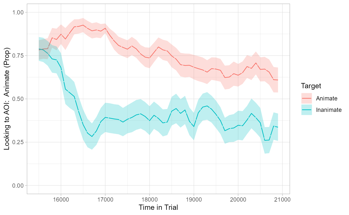

CPA in `{eyetrackingR}`

Continuing with the response_time dataframe, we jump to the “Bootstrapped cluster-based permutation analysis” of the original vignette.

Choosing the threshold

The original vignette uses the following heuristic of choosing a threshold:

num_sub <- length(unique((response_window_clean$ParticipantName)))
threshold_t <- qt(p = 1 - .05 / 2, df = num_sub - 1)
threshold_t
#> [1] 2.055529

How to choose a threshold is outside the scope of this article - we will simply use this value for both approaches.

In eyetrackingR, CPA is conducted in two steps:

Prepare data for CPA with make_time_cluster_data():

df_timeclust <- make_time_cluster_data(response_time,
  test = "t.test", paired = TRUE,
  predictor_column = "Target",
  threshold = threshold_t
)

This step computes the timewise statistics from the data and identifies the empirical clusters, which can be inspected with a plot() and summary() method:

plot(df_timeclust)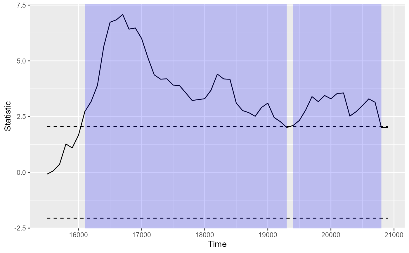

summary(df_timeclust)
#> Test Type:    t.test 
#> Predictor:    Target 
#> Formula:  Pair(Prop[Target == "Animate"], Prop[Target == "Inanimate"]) ~      1 
#> Summary of Clusters ======
#>   Cluster Direction SumStatistic StartTime EndTime
#> 1       1  Positive    132.29900     16100   19300
#> 2       2  Positive     42.31067     19400   20800

Run the permutation test on the cluster data with analyze_time_clusters():

system.time({
  clust_analysis <- analyze_time_clusters(
    df_timeclust,
    within_subj = TRUE,
    paired = TRUE,
    samples = 150,
    quiet = TRUE
  )
})
#>    user  system elapsed 
#>   19.63    0.10   29.61

This simulates a null distribution of cluster-mass statistics. The output, when printed, is essentially the output of summary(df_timeclust) with p-values (the Probability column)

clust_analysis
#> Test Type:    t.test 
#> Predictor:    Target 
#> Formula:  Pair(Prop[Target == "Animate"], Prop[Target == "Inanimate"]) ~      1 
#> Null Distribution   ====== 
#>  Mean:        -1.4815 
#>  2.5%:        -31.1268 
#> 97.5%:        17.9841 
#> Summary of Clusters ======
#>   Cluster Direction SumStatistic StartTime EndTime Probability
#> 1       1  Positive    132.29900     16100   19300 0.000000000
#> 2       2  Positive     42.31067     19400   20800 0.006666667

The null distribution (and the extremety of the empirical clusters in that context) can be visualized with a plot() method:

plot(clust_analysis)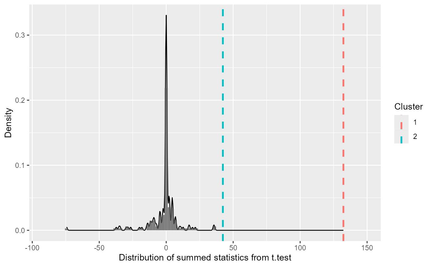

CPA in `{jlmerclusterperm}`

First, we set up jlmerclusterperm. For comparability, we use a single thread:

library(jlmerclusterperm)
options("jlmerclusterperm.nthreads" = 1)
system.time({
  # Note the overhead for initializing the Julia session
  jlmerclusterperm_setup()
})
#>    user  system elapsed 
#>    0.02    0.00   18.50

In {jlmerclusterpm}, CPA can also be conducted in two steps:

Make the specification object with make_jlmer_spec()

We first specify the formula, data, and grouping columns of the data. Instead of a paired t-test, we specify a linear model with the formula Prop ~ Target.

spec <- make_jlmer_spec(
  formula = Prop ~ Target,
  data = response_time,
  subject = "ParticipantName",
  trial = "Target",
  time = "TimeBin"
)
#> ! Dropping 37 rows with missing values.

The output prepares the data for CPA by subsetting it and applying the contrast coding schemes, among other things:

spec
#> ── jlmer specification ───────────────────────────────────────── <jlmer_spec> ──
#> Formula: Prop ~ 1 + TargetInanimate
#> Predictors:
#>   Target: TargetInanimate
#> Groupings:
#>   Subject: ParticipantName
#>   Trial: Target
#>   Time: TimeBin
#> Data:
#> # A tibble: 2,933 × 5
#>    Prop TargetInanimate ParticipantName Target  TimeBin
#>   <dbl>           <dbl> <fct>           <fct>     <dbl>
#> 1     0               0 ANCAT18         Animate     161
#> 2     0               0 ANCAT18         Animate     162
#> 3     1               0 ANCAT18         Animate     163
#> # ℹ 2,930 more rows
#> ────────────────────────────────────────────────────────────────────────────────

Run the permutation test with the specification using clusterpermute()

system.time({
  cpa <- clusterpermute(spec, threshold = threshold_t, nsim = 150)
})
#>    user  system elapsed 
#>    0.02    0.00   13.86

The same kinds of information are returned:

cpa
#> $null_cluster_dists
#> ── Null cluster-mass distribution (t > 2.05552943864287) ───────────────────────
#> TargetInanimate (n = 150)
#>   Mean (SD): -1.009 (11.03)
#>   Coverage intervals: 95% [-25.856, 27.183]
#> ────────────────────────────────────────────────────────────────────────────────
#> 
#> $empirical_clusters
#> ── Empirical clusters (t > 2.05552943864287) ─────────── <empirical_clusters> ──
#> TargetInanimate
#>   [161, 191]: -130.192 (p=0.0066)
#>   [194, 209]: -45.791 (p=0.0066)
#> ────────────────────────────────────────────────────────────────────────────────

The different pieces of information are available for further inspection using tidy(), which returns the dataframe underlying the summary:

null_distribution <- tidy(cpa$null_cluster_dists)
null_distribution
#> # A tibble: 150 × 6
#>    predictor       start   end length sum_statistic sim  
#>    <chr>           <dbl> <dbl>  <dbl>         <dbl> <fct>
#>  1 TargetInanimate    NA    NA     NA          0    001  
#>  2 TargetInanimate   208   209      2          5.09 002  
#>  3 TargetInanimate   197   200      4         -8.94 003  
#>  4 TargetInanimate   205   206      2         -4.32 004  
#>  5 TargetInanimate    NA    NA     NA          0    005  
#>  6 TargetInanimate   193   196      4        -10.8  006  
#>  7 TargetInanimate   187   193      7         19.3  007  
#>  8 TargetInanimate   177   180      4          9.34 008  
#>  9 TargetInanimate   159   161      3         -7.57 009  
#> 10 TargetInanimate    NA    NA     NA          0    010  
#> # ℹ 140 more rows

empirical_clusters <- tidy(cpa$empirical_clusters)
empirical_clusters
#> # A tibble: 2 × 7
#>   predictor       id    start   end length sum_statistic  pvalue
#>   <chr>           <fct> <dbl> <dbl>  <dbl>         <dbl>   <dbl>
#> 1 TargetInanimate 1       161   191     31        -130.  0.00662
#> 2 TargetInanimate 2       194   209     16         -45.8 0.00662

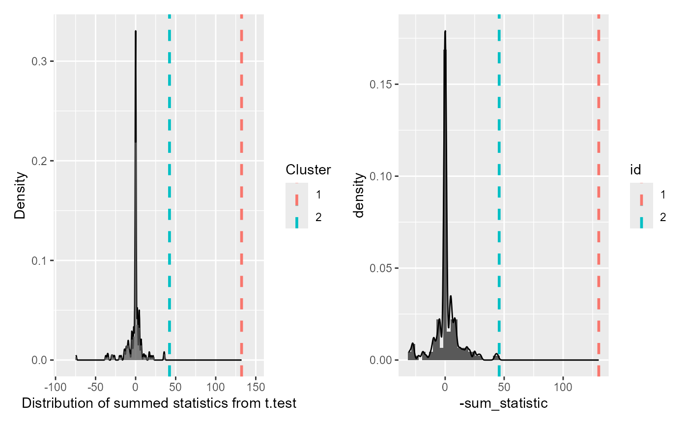
In contrast to eyetrackingR, jlmerclusterperm does not provide a custom plot() method. However, the same kinds of plots can be replicated with a few lines of ggplot code:

# We flip the sign of the statistic here for visual equivalence
cpa_plot <- null_distribution %>%
  ggplot(aes(-sum_statistic)) +
  geom_histogram(
    aes(y = after_stat(density)),
    binwidth = 3
  ) +
  geom_density() +
  geom_vline(
    aes(xintercept = -sum_statistic, color = id),
    data = empirical_clusters,
    linetype = 2,
    linewidth = 1
  )
cpa_plot

Note that while the sign of the clusters is (originally) flipped between the two approaches, this is a trivial difference that simply reflects the default choice of baseline in t.text() vs. regression contrasts. This can be addressed by setting contrasts prior to running the CPA (see related issue in another article).

Lastly, a side-by-side comparison of the results:

library(patchwork)
plot(clust_analysis) + cpa_plot

Performance

jlmerclusterperm scales easily to a higher number of simulations, especially for fixed-effects models:

system.time({
  clusterpermute(spec, threshold = threshold_t, nsim = 1000)
})
#>    user  system elapsed 
#>    0.01    0.00    8.31

While eyetrackingR does have an option for parallelization, it has limited support and is platform dependent. In contrast, jlmerclusterperm leverages Julia’s built-in multi-threading support which is more performant and consistent:

options("jlmerclusterperm.nthreads" = 7)
system.time({
  jlmerclusterperm_setup(restart = TRUE, verbose = FALSE)
})
#>    user  system elapsed 
#>    0.09    0.00   19.34

10,000 simulations with 7 threads:

system.time({
  clusterpermute(spec, threshold = threshold_t, nsim = 10000)
})
#>    user  system elapsed 
#>    0.17    0.40   36.39

Setup

CPA in {eyetrackingR}

CPA in {jlmerclusterperm}

Performance

CPA in `{eyetrackingR}`

CPA in `{jlmerclusterperm}`