This vignette showcases tidy() and other ways of
collecting jlmerclusterperm objects as tidy data.
See more tutorials and vignettes on the Articles page.
Setup
library(jlmerclusterperm)
jlmerclusterperm_setup(verbose = FALSE)
julia_progress(show = FALSE)
Minimal example data:
library(dplyr, warn.conflicts = FALSE)
library(ggplot2)
chickweights <- as_tibble(ChickWeight) %>%
  mutate(diet = forcats::fct_collapse(Diet, A = c(1, 3), B = c(2, 4))) %>%
  filter(Time %in% 0:20)
ggplot(chickweights, aes(Time, weight, color = diet)) +
  stat_summary(fun.args = list(mult = 1.96)) +
  stat_summary(geom = "line") +
  theme_minimal(base_size = 18)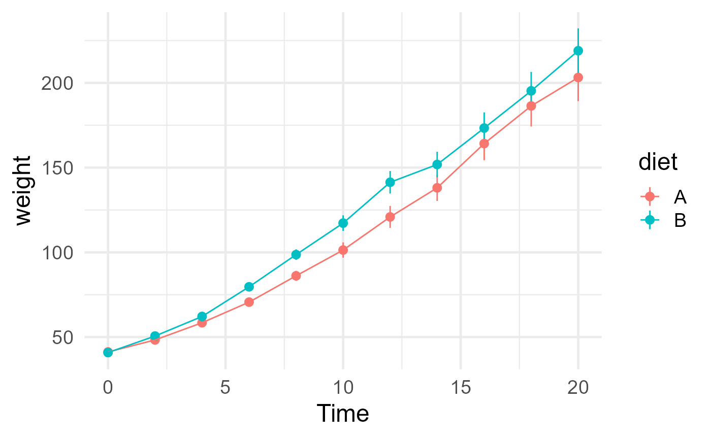
The jlmer specification object used for this showcase:
jlmer_spec <- make_jlmer_spec(
  formula = weight ~ diet + (1 | Chick), data = chickweights,
  subject = "Chick", time = "Time"
)
jlmer_spec
#> ── jlmer specification ───────────────────────────────────────── <jlmer_spec> ──
#> Formula: weight ~ 1 + dietB + (1 | Chick)
#> Predictors:
#>   diet: dietB
#> Groupings:
#>   Subject: Chick
#>   Trial:
#>   Time: Time
#> Data:
#> # A tibble: 533 × 4
#>   weight dietB Chick  Time
#>    <dbl> <dbl> <chr> <dbl>
#> 1     42     0 1         0
#> 2     51     0 1         2
#> 3     59     0 1         4
#> # ℹ 530 more rows
#> ────────────────────────────────────────────────────────────────────────────────
A tour of tidy() methods
All non-<data.frame> objects returned by
jlmerclusterperm functions have a tidy()
method to return a data frame representation of the object.
<timewise_statistics> objects
Functions compute_timewise_statistics() and
permute_timewise_statistics() return an object of class
<timewise_statistics>, which is an array of
statistics. Note that there isn’t a stylized print() method
for this class.
Instead, it is recommended to use tidy() to inspect the
results as a data frame where each statistic is represented as a
row.
In the case of compute_timewise_statistics(), the output
is a matrix (2D array) of predictor and time. Each dimension becomes a
column in the tidy() data:
empirical_statistics <- compute_timewise_statistics(jlmer_spec)
class(empirical_statistics)
#> [1] "timewise_statistics"
dim(empirical_statistics) # predictor x time
#> [1]  1 11
tidy(empirical_statistics)
#> # A tibble: 11 × 3
#>    predictor  time statistic
#>    <chr>     <dbl>     <dbl>
#>  1 dietB         0    -1.09
#>  2 dietB         2     2.29
#>  3 dietB         4     3.14
#>  4 dietB         6     4.01
#>  5 dietB         8     2.90
#>  6 dietB        10     2.44
#>  7 dietB        12     2.18
#>  8 dietB        14     1.26
#>  9 dietB        16     0.673
#> 10 dietB        18     0.532
#> 11 dietB        20     0.809
In the case of compute_timewise_statistics(), the output
is a 3D array of simulation, time, and predictor. Again, each dimension
becomes a column in the tidy() data:
null_statistics <- permute_timewise_statistics(jlmer_spec, nsim = 1000)
class(null_statistics)
#> [1] "timewise_statistics"
dim(null_statistics) # simulation x time x predictor
#> [1] 1000   11    1
tidy(null_statistics)
#> # A tibble: 11,000 × 4
#>    predictor  time statistic sim
#>    <chr>     <dbl>     <dbl> <fct>
#>  1 dietB         0   -0.309  0001
#>  2 dietB         0    2.10   0002
#>  3 dietB         0   -2.83   0003
#>  4 dietB         0   -0.568  0004
#>  5 dietB         0    2.10   0005
#>  6 dietB         0   -1.09   0006
#>  7 dietB         0   -0.830  0007
#>  8 dietB         0   -0.0515 0008
#>  9 dietB         0   -0.0515 0009
#> 10 dietB         0    0.206  0010
#> # ℹ 10,990 more rows
<empirical_clusters> objects
The <empirical_clusters> object returned by
extract_empirical_clusters() does have a print method
defined, which makes it easier on the eye:
empirical_clusters <- extract_empirical_clusters(empirical_statistics, threshold = 1)
class(empirical_clusters)
#> [1] "empirical_clusters"
empirical_clusters
#> ── Empirical clusters (t > 1) ────────────────────────── <empirical_clusters> ──
#> dietB
#>   [2, 14]: 18.231
#> ────────────────────────────────────────────────────────────────────────────────
The tidy() data frame representation also contains
information like length, which is the number of time points
that the cluster spans. The id variable uniquely identifies
a cluster within each predictor.
tidy(empirical_clusters)
#> # A tibble: 1 × 6
#>   predictor id    start   end length sum_statistic
#>   <chr>     <fct> <dbl> <dbl>  <dbl>         <dbl>
#> 1 dietB     1         2    14      7          18.2
<null_cluster_dists> objects
The <null_cluster_dists> object returned by
extract_null_cluster_dists() also has a print method
defined, which displays summary statistics:
null_cluster_dists <- extract_null_cluster_dists(null_statistics, threshold = 1)
class(null_cluster_dists)
#> [1] "null_cluster_dists"
null_cluster_dists
#> ── Null cluster-mass distribution (t > 1) ────────────── <null_cluster_dists> ──
#> dietB (n = 1000)
#>   Mean (SD): 0.014 (7.11)
#>   Coverage intervals: 95% [-15.360, 15.902]
#> ────────────────────────────────────────────────────────────────────────────────
The null distribution is constructed from the largest cluster-mass statistic observed in each of the bootstrapped permutations of the original data. In other words, each simulation contributes one sample to the null.
In the tidy() representation, each simulation of a
predictor represents a row. The sum_statistic column
represents the size of the largest cluster from each
simulation. When no clusters are found, the column is zero and values
for start, end, and length are
NA.
tidy(null_cluster_dists)
#> # A tibble: 1,000 × 6
#>    predictor start   end length sum_statistic sim
#>    <chr>     <dbl> <dbl>  <dbl>         <dbl> <fct>
#>  1 dietB         8    20      7         11.1  0001
#>  2 dietB         6    10      3          3.75 0002
#>  3 dietB        18    20      2          2.07 0003
#>  4 dietB         2    10      5          6.00 0004
#>  5 dietB         4    10      4          5.91 0005
#>  6 dietB        NA    NA     NA          0    0006
#>  7 dietB         8    20      7         12.2  0007
#>  8 dietB         2     8      4          5.29 0008
#>  9 dietB        NA    NA     NA          0    0009
#> 10 dietB        NA    NA     NA          0    0010
#> # ℹ 990 more rows
The output of tidy(null_statistics) and
tidy(null_cluster_dists) form a relational data. For
example, you can use left_join() to find the time wise
statistics of the permuted data with the most extreme cluster-mass
statistic:
largest_permuted_cluster <- tidy(null_cluster_dists) %>%
  slice(which.max(abs(sum_statistic))) %>%
  left_join(tidy(null_statistics), by = c("predictor", "sim"))
largest_permuted_cluster
#> # A tibble: 11 × 8
#>    predictor start   end length sum_statistic sim    time statistic
#>    <chr>     <dbl> <dbl>  <dbl>         <dbl> <fct> <dbl>     <dbl>
#>  1 dietB         2    20     10          29.4 0319      0     -1.09
#>  2 dietB         2    20     10          29.4 0319      2      1.67
#>  3 dietB         2    20     10          29.4 0319      4      2.56
#>  4 dietB         2    20     10          29.4 0319      6      2.97
#>  5 dietB         2    20     10          29.4 0319      8      3.47
#>  6 dietB         2    20     10          29.4 0319     10      3.54
#>  7 dietB         2    20     10          29.4 0319     12      3.49
#>  8 dietB         2    20     10          29.4 0319     14      3.54
#>  9 dietB         2    20     10          29.4 0319     16      3.05
#> 10 dietB         2    20     10          29.4 0319     18      2.65
#> 11 dietB         2    20     10          29.4 0319     20      2.48
Note that the sum_statistic is simply the sum of the
statistic values over the span of the largest cluster:
In other contexts
The output of calculate_clusters_pvalues() is just an
<empirical_clusters> object that has been augmented
with p-values:
tested_clusters <- calculate_clusters_pvalues(empirical_clusters, null_cluster_dists)
tested_clusters
#> ── Empirical clusters (t > 1) ────────────────────────── <empirical_clusters> ──
#> dietB
#>   [2, 14]: 18.231 (p=0.0270)
#> ────────────────────────────────────────────────────────────────────────────────
When available, p-values are returned as a column in the
tidy() data:
tidy(tested_clusters)
#> # A tibble: 1 × 7
#>   predictor id    start   end length sum_statistic pvalue
#>   <chr>     <fct> <dbl> <dbl>  <dbl>         <dbl>  <dbl>
#> 1 dietB     1         2    14      7          18.2  0.027
Note that the p-value for this cluster is 0.027 because there are 27 samples from the null that are as or more extreme than the observed:
tidy(null_cluster_dists) %>%
  filter(abs(sum_statistic) >= abs(tidy(tested_clusters)$sum_statistic))
#> # A tibble: 27 × 6
#>    predictor start   end length sum_statistic sim
#>    <chr>     <dbl> <dbl>  <dbl>         <dbl> <fct>
#>  1 dietB         0    20     11         -18.7 0072
#>  2 dietB         0    20     11         -19.4 0114
#>  3 dietB         6    20      8          19.0 0118
#>  4 dietB         0    20     11         -23.6 0137
#>  5 dietB         4    20      9         -21.7 0142
#>  6 dietB         2    20     10          24.7 0268
#>  7 dietB         4    20      9          22.7 0289
#>  8 dietB         2    20     10          29.4 0319
#>  9 dietB         2    20     10          26.4 0325
#> 10 dietB         4    20      9          26.5 0384
#> # ℹ 17 more rows
In the case of the one-fell-swoop function
clusterpermute(), the
<null_cluster_dists> object and the
<empirical_clusters> object are returned in a
list:
# Timing the entire process this time
system.time({
  full_test <- clusterpermute(jlmer_spec, threshold = 1, nsim = 1000, progress = FALSE)
})
#>    user  system elapsed
#>    0.00    0.03    1.66
full_test
#> $null_cluster_dists
#> ── Null cluster-mass distribution (t > 1) ────────────── <null_cluster_dists> ──
#> dietB (n = 1000)
#>   Mean (SD): 0.066 (7.61)
#>   Coverage intervals: 95% [-16.959, 17.216]
#> ────────────────────────────────────────────────────────────────────────────────
#>
#> $empirical_clusters
#> ── Empirical clusters (t > 1) ────────────────────────── <empirical_clusters> ──
#> dietB
#>   [2, 14]: 18.231 (p=0.0420)
#> ────────────────────────────────────────────────────────────────────────────────
You can tidy() the elements of this list with
lapply() or purrr::map():
lapply(full_test, tidy)
#> $null_cluster_dists
#> # A tibble: 1,000 × 6
#>    predictor start   end length sum_statistic sim
#>    <chr>     <dbl> <dbl>  <dbl>         <dbl> <fct>
#>  1 dietB        14    20      4         -5.26 0001
#>  2 dietB        14    20      4          9.22 0002
#>  3 dietB         6    20      8         11.8  0003
#>  4 dietB        NA    NA     NA          0    0004
#>  5 dietB        NA    NA     NA          0    0005
#>  6 dietB        16    20      3         -3.69 0006
#>  7 dietB        14    20      4          6.23 0007
#>  8 dietB        NA    NA     NA          0    0008
#>  9 dietB        12    20      5          5.38 0009
#> 10 dietB        NA    NA     NA          0    0010
#> # ℹ 990 more rows
#>
#> $empirical_clusters
#> # A tibble: 1 × 7
#>   predictor id    start   end length sum_statistic pvalue
#>   <chr>     <fct> <dbl> <dbl>  <dbl>         <dbl>  <dbl>
#> 1 dietB     1         2    14      7          18.2 0.0420
Tidying Julia model objects
Functions jlmer() and to_jlmer() return an
object of class <jlmer_mod>, which is a JuliaConnectoR
pointer to the Julia model object:
jlmer_mod <- to_jlmer(weight ~ diet + (1 | Chick), chickweights)
class(jlmer_mod)
#> [1] "jlmer_mod"        "JuliaStructProxy" "JuliaProxy"
jlmer_mod
#> <Julia object of type LinearMixedModel>
#> Variance components:
#>             Column    Variance Std.Dev.
#> Chick    (Intercept)   305.1809 17.4694
#> Residual              3854.0809 62.0812
#>  ──────────────────────────────────────────────────
#>                 Coef.  Std. Error      z  Pr(>|z|)
#> ──────────────────────────────────────────────────
#> (Intercept)  108.16       4.76331  22.71    <1e-99
#> dietB         12.2644     7.45319   1.65    0.0999
#> ──────────────────────────────────────────────────
You can use tidy() and glance() to return
information about the Julia model as a data frame:
tidy(jlmer_mod)
#> # A tibble: 4 × 7
#>   effect   group    term            estimate std.error statistic    p.value
#>   <chr>    <chr>    <chr>              <dbl>     <dbl>     <dbl>      <dbl>
#> 1 fixed    NA       (Intercept)        108.       4.76     22.7   3.83e-114
#> 2 fixed    NA       dietB               12.3      7.45      1.65  9.99e-  2
#> 3 ran_pars Chick    sd__(Intercept)     17.5     NA        NA    NA
#> 4 ran_pars Residual sd__Observation     62.1     NA        NA    NA
glance(jlmer_mod)
#> # A tibble: 1 × 8
#>    nobs    df sigma logLik   AIC   BIC deviance df.residual
#>   <int> <int> <dbl>  <dbl> <dbl> <dbl>    <dbl>       <int>
#> 1   533     4  62.1 -2972. 5952. 5969.    5944.         529
These mimic the behavior of the same methods from
broom/broom.mixed defined for
(g)lm/(g)lmer models:
library(lme4)
library(broom.mixed)
lmer_mod <- lmer(weight ~ diet + (1 | Chick), chickweights, REML = FALSE)
tidy(lmer_mod)
#> # A tibble: 4 × 6
#>   effect   group    term            estimate std.error statistic
#>   <chr>    <chr>    <chr>              <dbl>     <dbl>     <dbl>
#> 1 fixed    NA       (Intercept)        108.       4.76     22.7
#> 2 fixed    NA       dietB               12.3      7.45      1.65
#> 3 ran_pars Chick    sd__(Intercept)     17.5     NA        NA
#> 4 ran_pars Residual sd__Observation     62.1     NA        NA
glance(lmer_mod)
#> # A tibble: 1 × 7
#>    nobs sigma logLik   AIC   BIC deviance df.residual
#>   <int> <dbl>  <dbl> <dbl> <dbl>    <dbl>       <int>
#> 1   533  62.1 -2972. 5952. 5969.    5944.         529
Note that Julia MixedModels.jl
defaults to REML = FALSE, whereas it is TRUE
by default in lme4.