Inspect the value of variables from a method

Usage

ggtrace_inspect_vars(
  x,
  method,
  cond = 1L,
  at = "all",
  vars,
  by_var = TRUE,
  error = FALSE
)

Arguments

x

A ggplot object

method

A function or a ggproto method. The ggproto method may be specified using any of the following forms:

ggproto$method
namespace::ggproto$method
namespace:::ggproto$method

cond

When the return value should be inspected. Defaults to 1L.

at

Which steps in the method body the values of vars should be retrieved. Defaults to a special value all which is evaluated to all steps in the method body.

vars

A character vector of variable names

by_var

Boolean that controls the format of the output:

TRUE (default): returns a list of variables, with their values at each step. This also drops steps within a variable where the variable value has not changed from a previous step specified by at.
FALSE: returns a list of steps, where each element holds the value of vars at each step of at. Unchanged variable values are not dropped.

error

If TRUE, continues inspecting the method until the ggplot errors. This is useful for debugging but note that it can sometimes return incomplete output.

Value

A list of values of vars at each step at. Simplifies if vars and/or at is length-1.

Tracing context

When quoted expressions are passed to the cond or value argument of workflow functions they are evaluated in a special environment which we call the "tracing context".

The tracing context is "data-masked" (see rlang::eval_tidy()), and exposes an internal variable called ._counter_ which increments every time a function/method has been called by the ggplot object supplied to the x argument of workflow functions. For example, cond = quote(._counter_ == 1L) is evaluated as TRUE when the method is called for the first time. The cond argument also supports numeric shorthands like cond = 1L which evaluates to quote(._counter_ == 1L), and this is the default value of cond for all workflow functions that only return one value (e.g., ggtrace_capture_fn()). It is recommended to consult the output of ggtrace_inspect_n() and ggtrace_inspect_which() to construct expressions that condition on ._counter_.

For highjack functions like ggtrace_highjack_return(), the value about to be returned by the function/method can be accessed with returnValue() in the value argument. By default, value is set to quote(returnValue()) which simply evaluates to the return value, but directly computing on returnValue() to derive a different return value for the function/method is also possible.

Examples


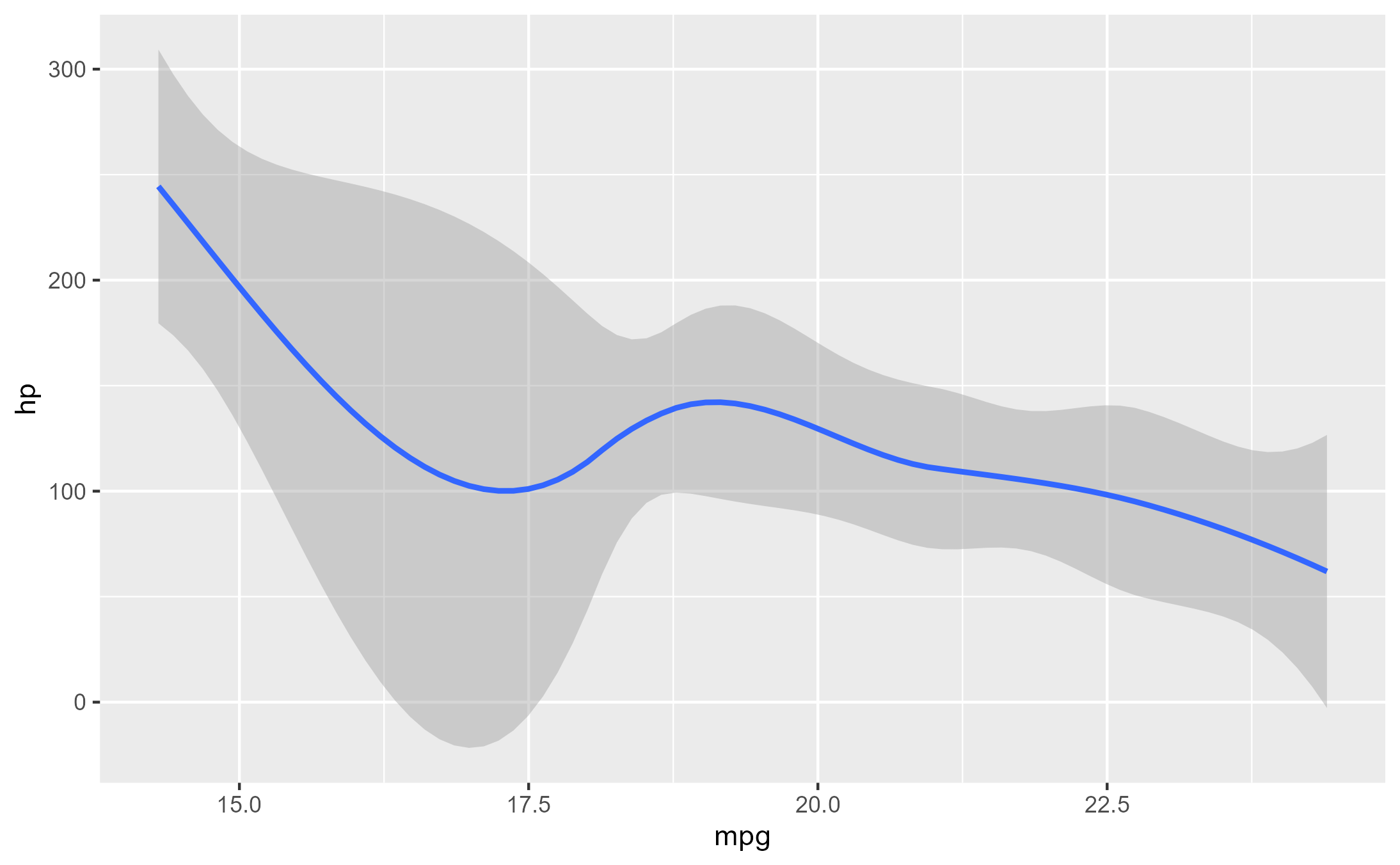
library(ggplot2)

p1 <- ggplot(mtcars[1:10,], aes(mpg, hp)) +
  geom_smooth()
p1
#> `geom_smooth()` using method = 'loess' and formula = 'y ~ x'


# The `data` variable is bound to two unique values in `compute_group` method:
ggtrace_inspect_vars(p1, StatSmooth$compute_group, vars = "data")
#> `geom_smooth()` using method = 'loess' and formula = 'y ~ x'
#> $Step1
#>       x   y PANEL group
#> 1  21.0 110     1    -1
#> 2  21.0 110     1    -1
#> 3  22.8  93     1    -1
#> 4  21.4 110     1    -1
#> 5  18.7 175     1    -1
#> 6  18.1 105     1    -1
#> 7  14.3 245     1    -1
#> 8  24.4  62     1    -1
#> 9  22.8  95     1    -1
#> 10 19.2 123     1    -1
#> 
#> $Step5
#>       x   y PANEL group weight
#> 1  21.0 110     1    -1      1
#> 2  21.0 110     1    -1      1
#> 3  22.8  93     1    -1      1
#> 4  21.4 110     1    -1      1
#> 5  18.7 175     1    -1      1
#> 6  18.1 105     1    -1      1
#> 7  14.3 245     1    -1      1
#> 8  24.4  62     1    -1      1
#> 9  22.8  95     1    -1      1
#> 10 19.2 123     1    -1      1
#> 

# Note that elements of this list capture the method's state upon entering a step,
# so "Step1" and "Step5" should be interpreted as the value of `data` at the start
# the method's execution (before "Step1") and its value as a result of running Step4
# (before "Step5"). Indeed, we see that the `weight` column is defined in Step4, so
# the data is flagged as changed at the start of Step5
ggbody(StatSmooth$compute_group)[[4]]
#> if (is.null(data$weight)) data$weight <- 1


# Comparing the "Steps" themselves can be useful
p2 <- p1 +
  scale_x_continuous(trans = "log") +
  scale_y_continuous(trans = "log")
p2
#> `geom_smooth()` using method = 'loess' and formula = 'y ~ x'


# Comparing the original plot to one with log-transformed scales reveals a change
# in data detected at the beginning of Step 14
names(ggtrace_inspect_vars(p1, ggplot2:::ggplot_build.ggplot, vars = "data"))
#> `geom_smooth()` using method = 'loess' and formula = 'y ~ x'
#> [1] "Step6"  "Step8"  "Step11" "Step12" "Step18" "Step29"
names(ggtrace_inspect_vars(p2, ggplot2:::ggplot_build.ggplot, vars = "data"))
#> `geom_smooth()` using method = 'loess' and formula = 'y ~ x'
#> [1] "Step6"  "Step8"  "Step11" "Step12" "Step13" "Step18" "Step29"

# We can pinpoint the calculation of scale transformations to Step 13:
ggbody(ggplot2:::ggplot_build.ggplot)[[13]]
#> scale_x <- function() scales$get_scales("x")


# With `by_vars = FALSE`, elements of the returned list are steps instead of values.
# Note that this does not drop unchanged values:
ggtrace_inspect_vars(p1, StatSmooth$compute_group, vars = "data", at = 1:6, by_var = FALSE)
#> `geom_smooth()` using method = 'loess' and formula = 'y ~ x'
#> $Step1
#> $Step1$data
#>       x   y PANEL group
#> 1  21.0 110     1    -1
#> 2  21.0 110     1    -1
#> 3  22.8  93     1    -1
#> 4  21.4 110     1    -1
#> 5  18.7 175     1    -1
#> 6  18.1 105     1    -1
#> 7  14.3 245     1    -1
#> 8  24.4  62     1    -1
#> 9  22.8  95     1    -1
#> 10 19.2 123     1    -1
#> 
#> 
#> $Step2
#> $Step2$data
#>       x   y PANEL group
#> 1  21.0 110     1    -1
#> 2  21.0 110     1    -1
#> 3  22.8  93     1    -1
#> 4  21.4 110     1    -1
#> 5  18.7 175     1    -1
#> 6  18.1 105     1    -1
#> 7  14.3 245     1    -1
#> 8  24.4  62     1    -1
#> 9  22.8  95     1    -1
#> 10 19.2 123     1    -1
#> 
#> 
#> $Step3
#> $Step3$data
#>       x   y PANEL group
#> 1  21.0 110     1    -1
#> 2  21.0 110     1    -1
#> 3  22.8  93     1    -1
#> 4  21.4 110     1    -1
#> 5  18.7 175     1    -1
#> 6  18.1 105     1    -1
#> 7  14.3 245     1    -1
#> 8  24.4  62     1    -1
#> 9  22.8  95     1    -1
#> 10 19.2 123     1    -1
#> 
#> 
#> $Step4
#> $Step4$data
#>       x   y PANEL group
#> 1  21.0 110     1    -1
#> 2  21.0 110     1    -1
#> 3  22.8  93     1    -1
#> 4  21.4 110     1    -1
#> 5  18.7 175     1    -1
#> 6  18.1 105     1    -1
#> 7  14.3 245     1    -1
#> 8  24.4  62     1    -1
#> 9  22.8  95     1    -1
#> 10 19.2 123     1    -1
#> 
#> 
#> $Step5
#> $Step5$data
#>       x   y PANEL group weight
#> 1  21.0 110     1    -1      1
#> 2  21.0 110     1    -1      1
#> 3  22.8  93     1    -1      1
#> 4  21.4 110     1    -1      1
#> 5  18.7 175     1    -1      1
#> 6  18.1 105     1    -1      1
#> 7  14.3 245     1    -1      1
#> 8  24.4  62     1    -1      1
#> 9  22.8  95     1    -1      1
#> 10 19.2 123     1    -1      1
#> 
#> 
#> $Step6
#> $Step6$data
#>       x   y PANEL group weight
#> 1  21.0 110     1    -1      1
#> 2  21.0 110     1    -1      1
#> 3  22.8  93     1    -1      1
#> 4  21.4 110     1    -1      1
#> 5  18.7 175     1    -1      1
#> 6  18.1 105     1    -1      1
#> 7  14.3 245     1    -1      1
#> 8  24.4  62     1    -1      1
#> 9  22.8  95     1    -1      1
#> 10 19.2 123     1    -1      1
#> 
#>