Debugging an extension package

This vignette is a detailed walk-through of an exploratory debugging workflow with {ggtrace}, using a Github issue opened on the {ggxmean} package by Gina Reynolds. We define “exploratory debugging” here as the process of learning and developing simultaneously, assuming little prior knowledge about ggplot internals.

Setup

library(ggtrace)
library(ggplot2)
theme_set(theme_minimal())

If you would like to follow along, you can install the version of the {ggxmean} package containing the bug that this vignette will address. We use devtools::dev_mode() here to install and inspect this version of {ggxmean} in development mode (except I skip installation here because I already have that version in my dev directory).

library(devtools)
#> Loading required package: usethis

# Current installation version
devtools::package_info("ggxmean", FALSE, FALSE)$source
#> [1] "local"

# Activate development mode
devtools::dev_mode(on = TRUE, path = getOption("devtools.path"))
#> ✔ Dev mode: ON

# devtools::install_github("EvaMaeRey/ggxmean@cbb909c")

# Prior version installed for dev mode
devtools::package_info("ggxmean", FALSE, FALSE)$source
#> [1] "Github (EvaMaeRey/ggxmean@cbb909cee7d4f0a4395722020a75330641e5f54c)"

library(ggxmean)

I’ve also attached the code relevant to the issue at hand here, if you would like to familiarize yourself with it before we begin (though we do not assume this as prior knowledge here).

Relevant code from {ggxmean}

# https://github.com/EvaMaeRey/ggxmean/blob/cbb909cee7d4f0a4395722020a75330641e5f54c/R/geom_x_line.R 
GeomXline <- ggplot2::ggproto("GeomXline", ggplot2::Geom,
                     draw_panel = function(data, panel_params, coord) {
                       ranges <- coord$backtransform_range(panel_params)
                       data$x    <- data$x
                       data$xend <- data$x
                       data$y    <- ranges$y[1]
                       data$yend <- ranges$y[2]
                       GeomSegment$draw_panel(unique(data), panel_params, coord)
                     },
                     default_aes = ggplot2::aes(colour = "black", size = 0.5,
                                       linetype = 1, alpha = NA),
                     required_aes = "x",
                     draw_key = ggplot2::draw_key_vline
)

# https://github.com/EvaMaeRey/ggxmean/blob/cbb909cee7d4f0a4395722020a75330641e5f54c/R/geom_x_mean.R
StatXmean <- ggplot2::ggproto("StatXmean",
                              ggplot2::Stat,
                              compute_group = function(data, scales) {
                                data.frame(x = mean(data$x))
                              },
                              required_aes = c("x")
)

geom_x_mean <- function(mapping = NULL, data = NULL,
                        position = "identity", na.rm = FALSE, show.legend = NA,
                        inherit.aes = TRUE, ...) {
  ggplot2::layer(
    stat = StatXmean, geom = GeomXline, data = data, mapping = mapping,
    position = position, show.legend = show.legend, inherit.aes = inherit.aes,
    params = list(na.rm = na.rm, ...)
  )
}

Introduction of the issue

{ggxmean} is a {ggplot2} extension package that offers many features, including the layer geom_x_mean() which can be used to draw a line at the mean value of the variable represented by the x-axis.

ggplot(mpg, aes(x = hwy)) +
  geom_histogram() +
  geom_x_mean()
#> `stat_bin()` using `bins = 30`. Pick better value with `binwidth`.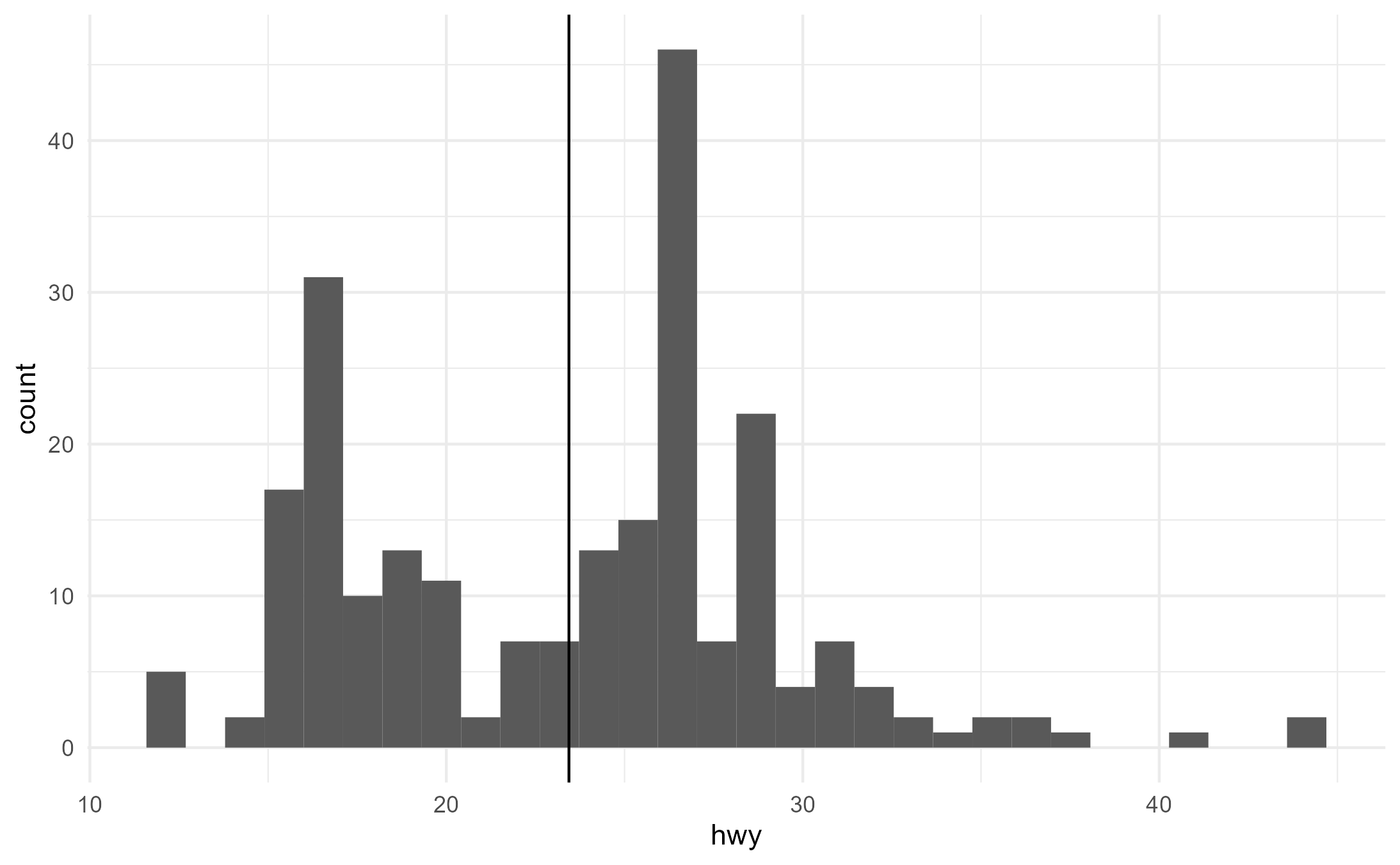

geom_x_mean() works smoothly with groups and facets, as we might expect from our experience with ggplot.

ggplot(mpg, aes(x = hwy, group = drv)) +
  geom_histogram() +
  geom_x_mean() +
  facet_wrap(~drv)
#> `stat_bin()` using `bins = 30`. Pick better value with `binwidth`.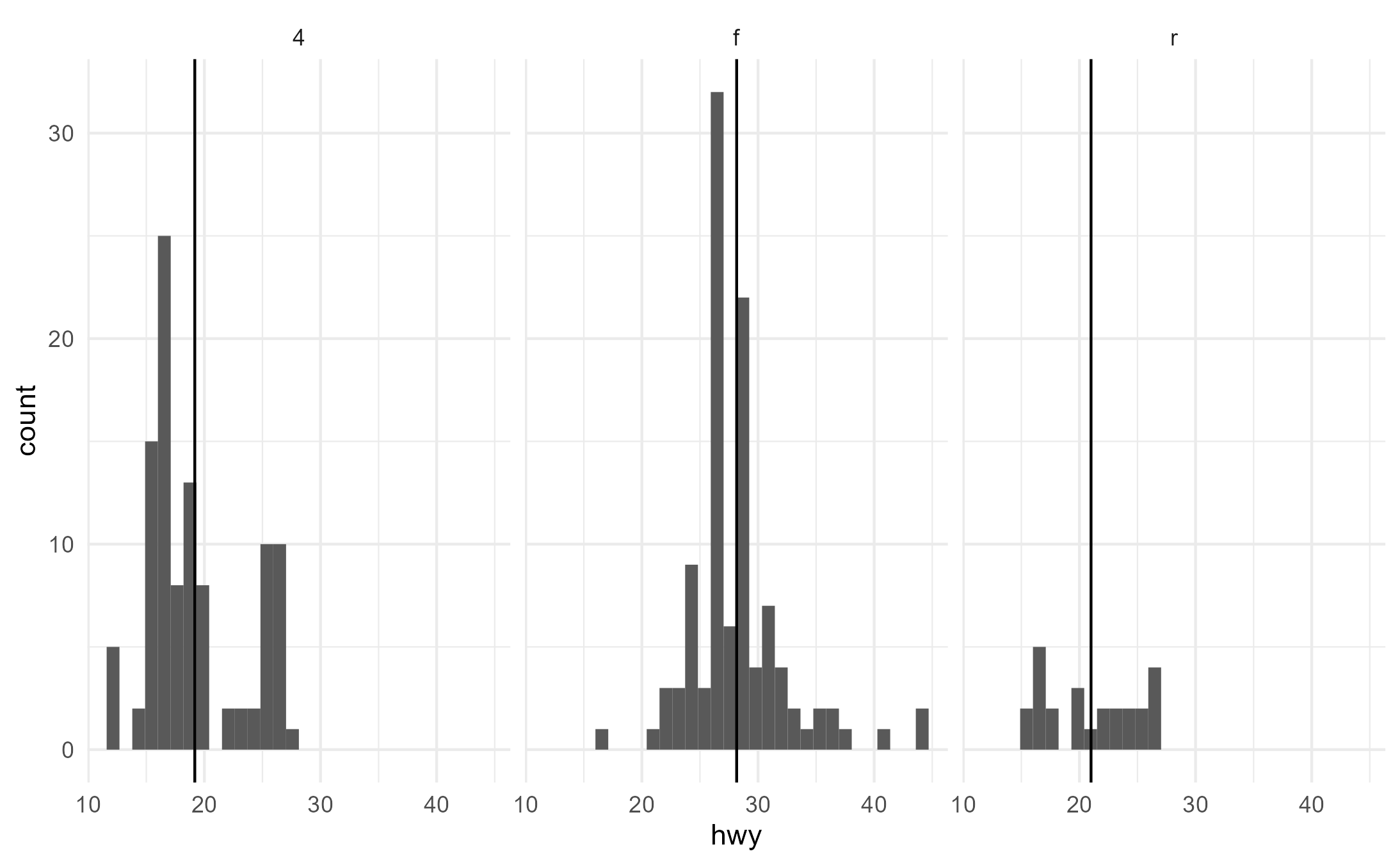

However, something somewhat unexpected happens when we pass map a discrete variable to an aesthetic that is not understandable by geom_x_mean(). Despite the fact that the lines do not understand the fill aesthetic, the aesthetic mapping of fill = drv nevertheless highjacks the calculation of grouping for geom_x_mean().

ggplot(mpg, aes(x = hwy, fill = drv)) +
  geom_histogram() +
  geom_x_mean()
#> `stat_bin()` using `bins = 30`. Pick better value with `binwidth`.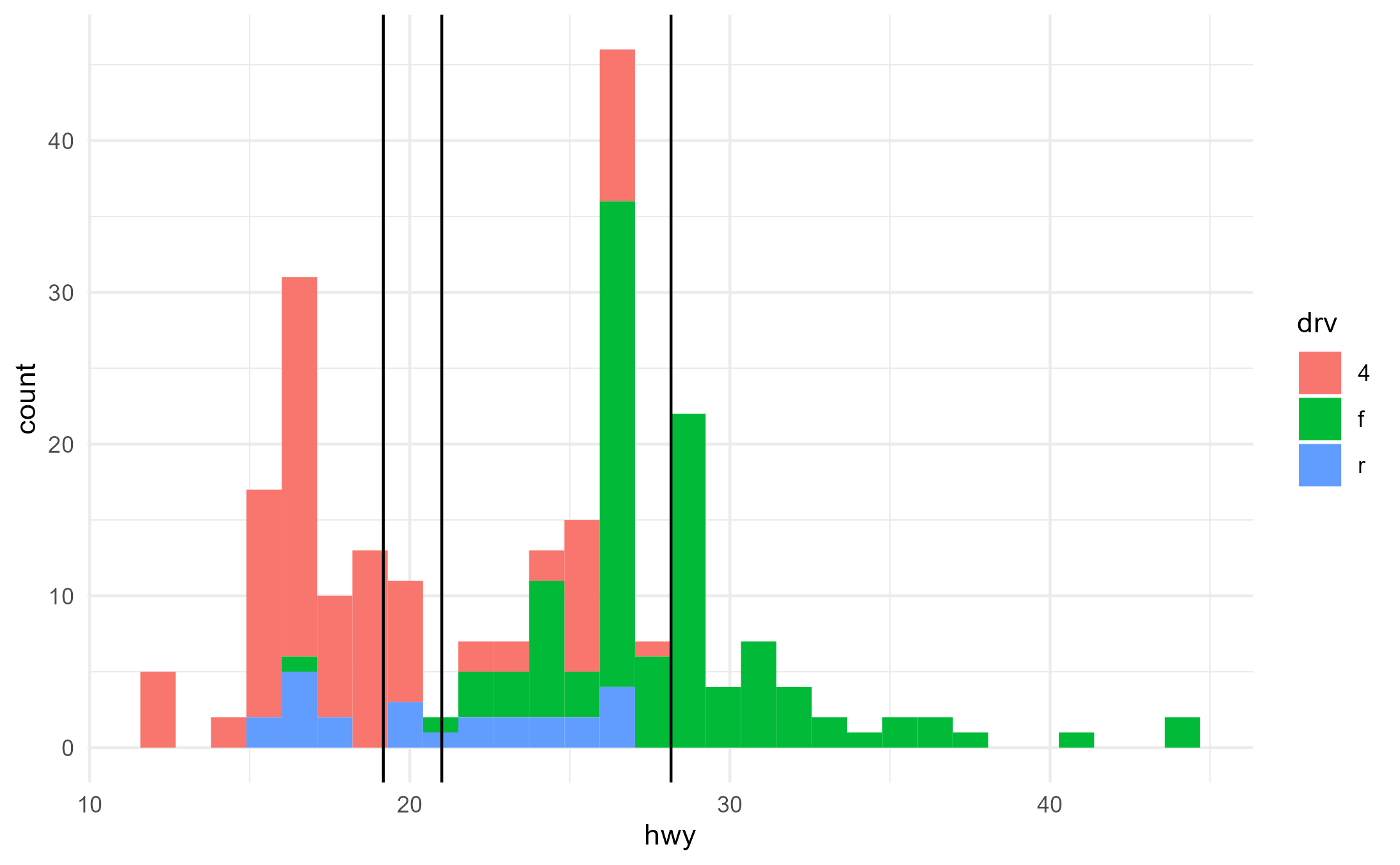

Making a reprex

To isolate the problem, let’s remove geom_histogram() from the examples.

Here is a minimal reprex (reproducible example) of the issue:

ggplot(mpg) +
  aes(x = hwy, fill = drv) +
  geom_x_mean()

We can pinpoint and formalize the issue with the help of layer_data(). We see that in both our expected group = drv and unexpected fill = drv cases, we end up with three unique groups (lines) as indicated by the values in the group column.

p <- ggplot(mpg) +
  aes(x = hwy) +
  geom_x_mean()
layer_data(p + aes(group = drv))
#>          x group PANEL colour size linetype alpha
#> 1 19.17476     1     1  black  0.5        1    NA
#> 2 28.16038     2     1  black  0.5        1    NA
#> 3 21.00000     3     1  black  0.5        1    NA
layer_data(p + aes(fill = drv))
#>      fill        x PANEL group colour size linetype alpha
#> 1 #F8766D 19.17476     1     1  black  0.5        1    NA
#> 2 #00BA38 28.16038     1     2  black  0.5        1    NA
#> 3 #619CFF 21.00000     1     3  black  0.5        1    NA

Expected cases

Here, we correctly get groups for each category of drv because lines understand the color aesthetic.

p + aes(color = drv)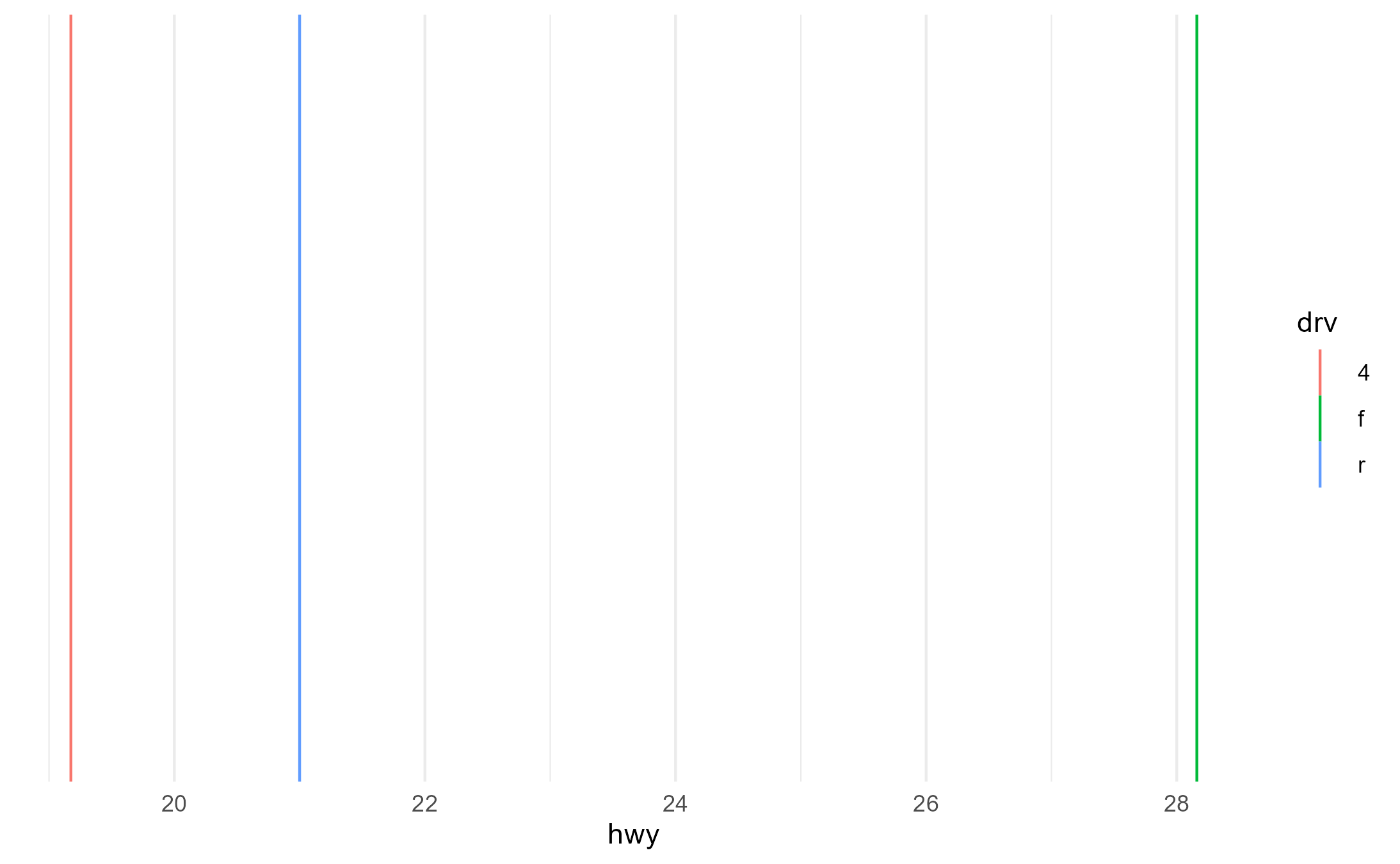

layer_data(p + aes(color = drv))$group
#> [1] 1 2 3

We also correctly get groups for each category of drv when we set the group aesthetic explicitly.

p + aes(group = drv)

layer_data(p + aes(group = drv))$group
#> [1] 1 2 3

Unexpected cases

Here, we’d only like there to be 1 group/line because lines don’t understand the shape aesthetic

p + aes(shape = drv)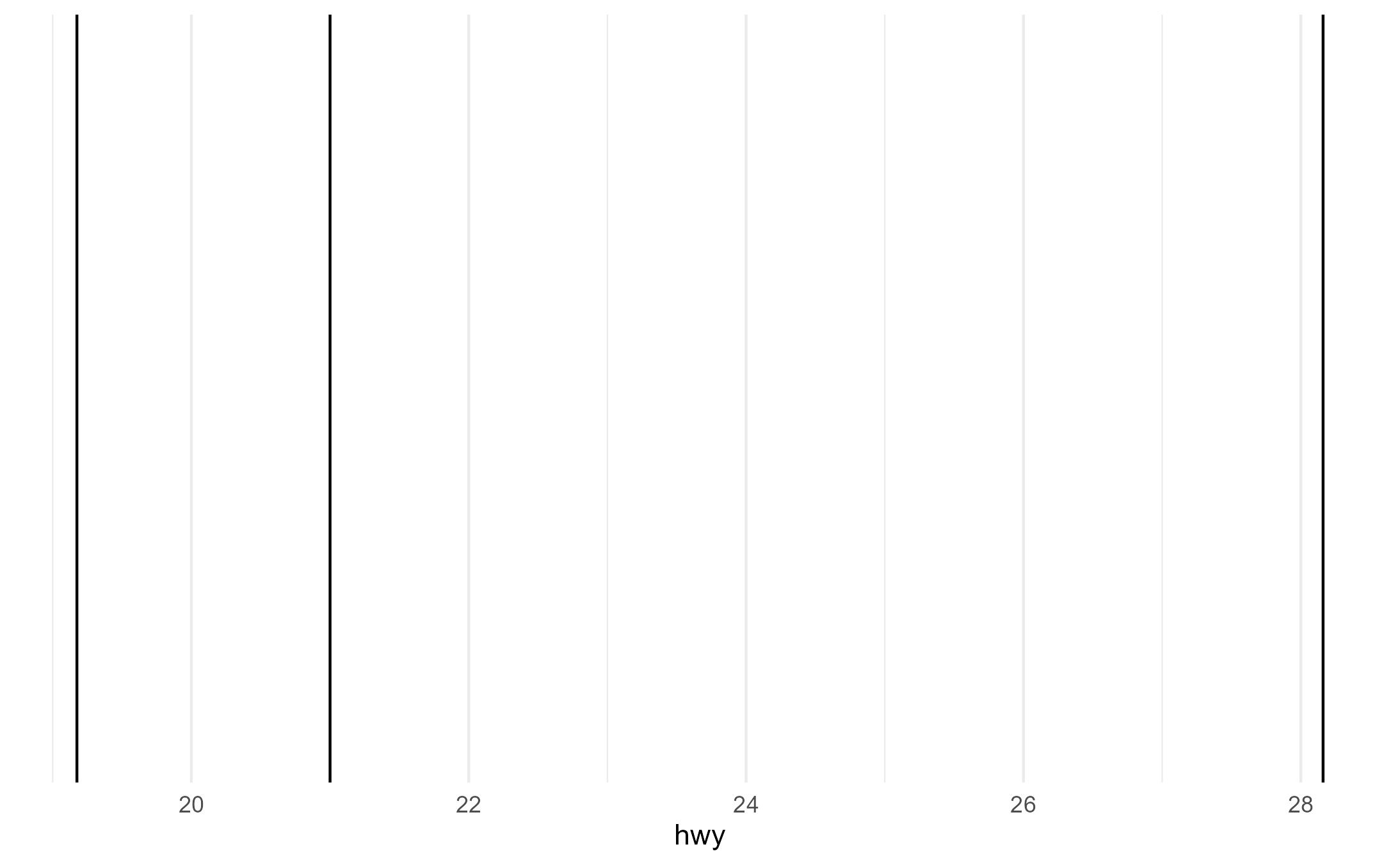

layer_data(p + aes(shape = drv))$group
#> [1] 1 2 3

Here, we’d only like there to be 3 groups for drv mapped to color. Categories in the fl variable should not interact with drv in the creation of the groups because lines don’t understand the fill aesthetic.

p + aes(fill = fl, color = drv)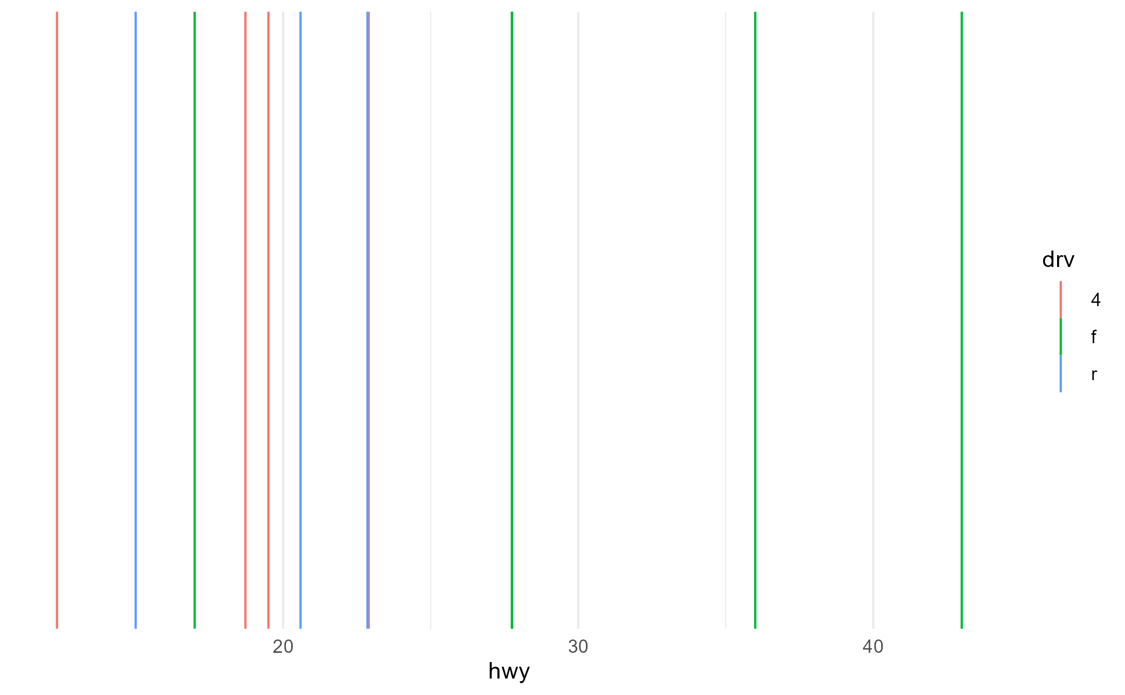

layer_data(p + aes(fill = fl, color = drv))$group
#>  [1]  1  2  3  4  5  6  7  8  9 10 11 12

Debugging the issue with {ggtrace}

Step 1 - Locating the problem

1.1 Starting at ggplot_build()

As our very first step, let’s see where the groups are being calculated and added to the data by inspecting ggplot_build(), the main engine behind ggplot. For exploratory debugging of ggplot internals, inspecting the data transformation pipeline in ggplot_build() is often the best place to start.

If this is your first exposure to ggplot_build(), you just need to know that its output is basically what’s returned by the layer_data() function that we demoed above.

layer_data
#> function (plot, i = 1L) 
#> {
#>     ggplot_build(plot)$data[[i]]
#> }
#> <bytecode: 0x0000020c05f5ffe8>
#> <environment: namespace:ggplot2>

We use ggbody() function from {ggtrace} to grab the body of ggplot_build() as a list, and, with some metaprogramming with rlang, pick out the steps where the data gets transformed. Note that the syntax ggplot2:::ggplot_build.ggplot reflects the fact that ggplot_build() is an S3 generic defined for the class <<ggplot>>.

build_pipeline <- ggbody(ggplot2:::ggplot_build.ggplot)
data_assigns <- sapply(build_pipeline,
  function(x) {
    rlang::is_call(x) &&
      !is.null(rlang::call_name(x)) && 
      rlang::call_name(x) == "<-" &&
      rlang::call_args(x)[[1]] == "data"
  }
)
which(data_assigns) # Steps of the build pipeline where data is transformed
#>  [1]  8  9 11 12 13 17 18 19 21 22 26 29 30 31

You can inspect the source code for ggplot_build() on the ggplot2 Github repo, and the output of ggbody(ggplot2:::ggplot_build.ggplot) is also available below:

Body of ggplot_build()

ggbody(ggplot2:::ggplot_build.ggplot)
#> [[1]]
#> `{`
#> 
#> [[2]]
#> plot <- plot_clone(plot)
#> 
#> [[3]]
#> if (length(plot$layers) == 0) {
#>     plot <- plot + geom_blank()
#> }
#> 
#> [[4]]
#> layers <- plot$layers
#> 
#> [[5]]
#> layer_data <- lapply(layers, function(y) y$layer_data(plot$data))
#> 
#> [[6]]
#> scales <- plot$scales
#> 
#> [[7]]
#> by_layer <- function(f) {
#>     out <- vector("list", length(data))
#>     for (i in seq_along(data)) {
#>         out[[i]] <- f(l = layers[[i]], d = data[[i]])
#>     }
#>     out
#> }
#> 
#> [[8]]
#> data <- layer_data
#> 
#> [[9]]
#> data <- by_layer(function(l, d) l$setup_layer(d, plot))
#> 
#> [[10]]
#> layout <- create_layout(plot$facet, plot$coordinates)
#> 
#> [[11]]
#> data <- layout$setup(data, plot$data, plot$plot_env)
#> 
#> [[12]]
#> data <- by_layer(function(l, d) l$compute_aesthetics(d, plot))
#> 
#> [[13]]
#> data <- lapply(data, scales_transform_df, scales = scales)
#> 
#> [[14]]
#> scale_x <- function() scales$get_scales("x")
#> 
#> [[15]]
#> scale_y <- function() scales$get_scales("y")
#> 
#> [[16]]
#> layout$train_position(data, scale_x(), scale_y())
#> 
#> [[17]]
#> data <- layout$map_position(data)
#> 
#> [[18]]
#> data <- by_layer(function(l, d) l$compute_statistic(d, layout))
#> 
#> [[19]]
#> data <- by_layer(function(l, d) l$map_statistic(d, plot))
#> 
#> [[20]]
#> scales_add_missing(plot, c("x", "y"), plot$plot_env)
#> 
#> [[21]]
#> data <- by_layer(function(l, d) l$compute_geom_1(d))
#> 
#> [[22]]
#> data <- by_layer(function(l, d) l$compute_position(d, layout))
#> 
#> [[23]]
#> layout$reset_scales()
#> 
#> [[24]]
#> layout$train_position(data, scale_x(), scale_y())
#> 
#> [[25]]
#> layout$setup_panel_params()
#> 
#> [[26]]
#> data <- layout$map_position(data)
#> 
#> [[27]]
#> npscales <- scales$non_position_scales()
#> 
#> [[28]]
#> if (npscales$n() > 0) {
#>     lapply(data, scales_train_df, scales = npscales)
#>     data <- lapply(data, scales_map_df, scales = npscales)
#> }
#> 
#> [[29]]
#> data <- by_layer(function(l, d) l$compute_geom_2(d))
#> 
#> [[30]]
#> data <- by_layer(function(l, d) l$finish_statistics(d))
#> 
#> [[31]]
#> data <- layout$finish_data(data)
#> 
#> [[32]]
#> plot$labels$alt <- get_alt_text(plot)
#> 
#> [[33]]
#> structure(list(data = data, layout = layout, plot = plot), class = "ggplot_built")

After each data transformation step (steps + 1L), let’s log the data for the first (and only) layer of our reprex plot.

ggtrace(
  method = ggplot2:::ggplot_build.ggplot,
  trace_steps = which(data_assigns) + 1, # After each data transformation step ...
  trace_exprs = quote(data[[1]]),        # ... return the data for the first layer
  verbose = FALSE
)
#> `ggplot2:::ggplot_build.ggplot` now being traced.

# plot not printed for space
p + aes(fill = drv)
#> Triggering trace on `ggplot2:::ggplot_build.ggplot`
#> Untracing `ggplot2:::ggplot_build.ggplot` on exit.

tracedump1 <- last_ggtrace()

Here, tracedump1 is a list of what data looked like after each data-transformation step inside ggplot_build(). It’s a list of data frames and there’s a lot here, but here’s what it looks like after it’s been cleaned up with tibble::as_tibble()

The evaluated trace expressions captured by last_ggtrace()

lapply(tracedump1, tibble::as_tibble)
#> [[1]]
#> # A tibble: 234 × 11
#>    manufacturer model      displ  year   cyl trans drv     cty   hwy fl    class
#>    <chr>        <chr>      <dbl> <int> <int> <chr> <chr> <int> <int> <chr> <chr>
#>  1 audi         a4           1.8  1999     4 auto… f        18    29 p     comp…
#>  2 audi         a4           1.8  1999     4 manu… f        21    29 p     comp…
#>  3 audi         a4           2    2008     4 manu… f        20    31 p     comp…
#>  4 audi         a4           2    2008     4 auto… f        21    30 p     comp…
#>  5 audi         a4           2.8  1999     6 auto… f        16    26 p     comp…
#>  6 audi         a4           2.8  1999     6 manu… f        18    26 p     comp…
#>  7 audi         a4           3.1  2008     6 auto… f        18    27 p     comp…
#>  8 audi         a4 quattro   1.8  1999     4 manu… 4        18    26 p     comp…
#>  9 audi         a4 quattro   1.8  1999     4 auto… 4        16    25 p     comp…
#> 10 audi         a4 quattro   2    2008     4 manu… 4        20    28 p     comp…
#> # … with 224 more rows
#> # ℹ Use `print(n = ...)` to see more rows
#> 
#> [[2]]
#> # A tibble: 234 × 11
#>    manufacturer model      displ  year   cyl trans drv     cty   hwy fl    class
#>    <chr>        <chr>      <dbl> <int> <int> <chr> <chr> <int> <int> <chr> <chr>
#>  1 audi         a4           1.8  1999     4 auto… f        18    29 p     comp…
#>  2 audi         a4           1.8  1999     4 manu… f        21    29 p     comp…
#>  3 audi         a4           2    2008     4 manu… f        20    31 p     comp…
#>  4 audi         a4           2    2008     4 auto… f        21    30 p     comp…
#>  5 audi         a4           2.8  1999     6 auto… f        16    26 p     comp…
#>  6 audi         a4           2.8  1999     6 manu… f        18    26 p     comp…
#>  7 audi         a4           3.1  2008     6 auto… f        18    27 p     comp…
#>  8 audi         a4 quattro   1.8  1999     4 manu… 4        18    26 p     comp…
#>  9 audi         a4 quattro   1.8  1999     4 auto… 4        16    25 p     comp…
#> 10 audi         a4 quattro   2    2008     4 manu… 4        20    28 p     comp…
#> # … with 224 more rows
#> # ℹ Use `print(n = ...)` to see more rows
#> 
#> [[3]]
#> # A tibble: 234 × 12
#>    manufactu…¹ model displ  year   cyl trans drv     cty   hwy fl    class PANEL
#>    <chr>       <chr> <dbl> <int> <int> <chr> <chr> <int> <int> <chr> <chr> <fct>
#>  1 audi        a4      1.8  1999     4 auto… f        18    29 p     comp… 1    
#>  2 audi        a4      1.8  1999     4 manu… f        21    29 p     comp… 1    
#>  3 audi        a4      2    2008     4 manu… f        20    31 p     comp… 1    
#>  4 audi        a4      2    2008     4 auto… f        21    30 p     comp… 1    
#>  5 audi        a4      2.8  1999     6 auto… f        16    26 p     comp… 1    
#>  6 audi        a4      2.8  1999     6 manu… f        18    26 p     comp… 1    
#>  7 audi        a4      3.1  2008     6 auto… f        18    27 p     comp… 1    
#>  8 audi        a4 q…   1.8  1999     4 manu… 4        18    26 p     comp… 1    
#>  9 audi        a4 q…   1.8  1999     4 auto… 4        16    25 p     comp… 1    
#> 10 audi        a4 q…   2    2008     4 manu… 4        20    28 p     comp… 1    
#> # … with 224 more rows, and abbreviated variable name ¹​manufacturer
#> # ℹ Use `print(n = ...)` to see more rows
#> 
#> [[4]]
#> # A tibble: 234 × 4
#>    fill      x PANEL group
#>    <chr> <int> <fct> <int>
#>  1 f        29 1         2
#>  2 f        29 1         2
#>  3 f        31 1         2
#>  4 f        30 1         2
#>  5 f        26 1         2
#>  6 f        26 1         2
#>  7 f        27 1         2
#>  8 4        26 1         1
#>  9 4        25 1         1
#> 10 4        28 1         1
#> # … with 224 more rows
#> # ℹ Use `print(n = ...)` to see more rows
#> 
#> [[5]]
#> # A tibble: 234 × 4
#>    fill      x PANEL group
#>    <chr> <int> <fct> <int>
#>  1 f        29 1         2
#>  2 f        29 1         2
#>  3 f        31 1         2
#>  4 f        30 1         2
#>  5 f        26 1         2
#>  6 f        26 1         2
#>  7 f        27 1         2
#>  8 4        26 1         1
#>  9 4        25 1         1
#> 10 4        28 1         1
#> # … with 224 more rows
#> # ℹ Use `print(n = ...)` to see more rows
#> 
#> [[6]]
#> # A tibble: 234 × 4
#>    fill      x PANEL group
#>    <chr> <dbl> <fct> <int>
#>  1 f        29 1         2
#>  2 f        29 1         2
#>  3 f        31 1         2
#>  4 f        30 1         2
#>  5 f        26 1         2
#>  6 f        26 1         2
#>  7 f        27 1         2
#>  8 4        26 1         1
#>  9 4        25 1         1
#> 10 4        28 1         1
#> # … with 224 more rows
#> # ℹ Use `print(n = ...)` to see more rows
#> 
#> [[7]]
#> # A tibble: 3 × 4
#>       x fill  PANEL group
#>   <dbl> <chr> <fct> <int>
#> 1  19.2 4     1         1
#> 2  28.2 f     1         2
#> 3  21   r     1         3
#> 
#> [[8]]
#> # A tibble: 3 × 4
#>       x fill  PANEL group
#>   <dbl> <chr> <fct> <int>
#> 1  19.2 4     1         1
#> 2  28.2 f     1         2
#> 3  21   r     1         3
#> 
#> [[9]]
#> # A tibble: 3 × 4
#>       x fill  PANEL group
#>   <dbl> <chr> <fct> <int>
#> 1  19.2 4     1         1
#> 2  28.2 f     1         2
#> 3  21   r     1         3
#> 
#> [[10]]
#> # A tibble: 3 × 4
#>       x fill  PANEL group
#>   <dbl> <chr> <fct> <int>
#> 1  19.2 4     1         1
#> 2  28.2 f     1         2
#> 3  21   r     1         3
#> 
#> [[11]]
#> # A tibble: 3 × 4
#>       x fill  PANEL group
#>   <dbl> <chr> <fct> <int>
#> 1  19.2 4     1         1
#> 2  28.2 f     1         2
#> 3  21   r     1         3
#> 
#> [[12]]
#> # A tibble: 3 × 8
#>   fill        x PANEL group colour  size linetype alpha
#>   <chr>   <dbl> <fct> <int> <chr>  <dbl>    <dbl> <lgl>
#> 1 #F8766D  19.2 1         1 black    0.5        1 NA   
#> 2 #00BA38  28.2 1         2 black    0.5        1 NA   
#> 3 #619CFF  21   1         3 black    0.5        1 NA   
#> 
#> [[13]]
#> # A tibble: 3 × 8
#>   fill        x PANEL group colour  size linetype alpha
#>   <chr>   <dbl> <fct> <int> <chr>  <dbl>    <dbl> <lgl>
#> 1 #F8766D  19.2 1         1 black    0.5        1 NA   
#> 2 #00BA38  28.2 1         2 black    0.5        1 NA   
#> 3 #619CFF  21   1         3 black    0.5        1 NA   
#> 
#> [[14]]
#> # A tibble: 3 × 8
#>   fill        x PANEL group colour  size linetype alpha
#>   <chr>   <dbl> <fct> <int> <chr>  <dbl>    <dbl> <lgl>
#> 1 #F8766D  19.2 1         1 black    0.5        1 NA   
#> 2 #00BA38  28.2 1         2 black    0.5        1 NA   
#> 3 #619CFF  21   1         3 black    0.5        1 NA

We can now map over every element of the list to see where the group column was first present.

group_present1 <- sapply(tracedump1, function(x) {
  "group" %in% colnames(x) && sort(unique(x$group)) == 1:3
})
#> Warning in "group" %in% colnames(x) && sort(unique(x$group)) == 1:3: 'length(x)
#> = 3 > 1' in coercion to 'logical(1)'

#> Warning in "group" %in% colnames(x) && sort(unique(x$group)) == 1:3: 'length(x)
#> = 3 > 1' in coercion to 'logical(1)'

#> Warning in "group" %in% colnames(x) && sort(unique(x$group)) == 1:3: 'length(x)
#> = 3 > 1' in coercion to 'logical(1)'

#> Warning in "group" %in% colnames(x) && sort(unique(x$group)) == 1:3: 'length(x)
#> = 3 > 1' in coercion to 'logical(1)'

#> Warning in "group" %in% colnames(x) && sort(unique(x$group)) == 1:3: 'length(x)
#> = 3 > 1' in coercion to 'logical(1)'

#> Warning in "group" %in% colnames(x) && sort(unique(x$group)) == 1:3: 'length(x)
#> = 3 > 1' in coercion to 'logical(1)'

#> Warning in "group" %in% colnames(x) && sort(unique(x$group)) == 1:3: 'length(x)
#> = 3 > 1' in coercion to 'logical(1)'

#> Warning in "group" %in% colnames(x) && sort(unique(x$group)) == 1:3: 'length(x)
#> = 3 > 1' in coercion to 'logical(1)'

#> Warning in "group" %in% colnames(x) && sort(unique(x$group)) == 1:3: 'length(x)
#> = 3 > 1' in coercion to 'logical(1)'

#> Warning in "group" %in% colnames(x) && sort(unique(x$group)) == 1:3: 'length(x)
#> = 3 > 1' in coercion to 'logical(1)'

#> Warning in "group" %in% colnames(x) && sort(unique(x$group)) == 1:3: 'length(x)
#> = 3 > 1' in coercion to 'logical(1)'
group_present1
#>  [1] FALSE FALSE FALSE  TRUE  TRUE  TRUE  TRUE  TRUE  TRUE  TRUE  TRUE  TRUE
#> [13]  TRUE  TRUE

Step 12 of ggplot_build() is where group first appears. We suspect that that’s where group is computed and assigned

which(data_assigns)[min(which(group_present1))]
#> [1] 12
ggbody(ggplot2:::ggplot_build.ggplot)[[12]]
#> data <- by_layer(function(l, d) l$compute_aesthetics(d, plot))

The code from Step 12 of ggplot_build() calls the compute_aesthetics method of each layer l. The by_layer() function defined in Step 7 of ggplot_build() is what’s doing this.

The internal function by_layer()

ggbody(ggplot2:::ggplot_build.ggplot)[[7]]
#> by_layer <- function(f) {
#>     out <- vector("list", length(data))
#>     for (i in seq_along(data)) {
#>         out[[i]] <- f(l = layers[[i]], d = data[[i]])
#>     }
#>     out
#> }

1.2 Digging deeper into Layer$compute_aesthetics()

At this point we realize that we have to go a little deeper than ggplot_build(). We need to inspect Layer$compute_aesthetics - the compute_aesthetics method of the Layer ggproto.

(Check out the quick aside on the Layer ggproto below if this is your first time encountering it, but for the purposes of this vignette you just need to know that Layer$compute_aesthetics is a function called inside ggplot_build() where we think group is being calculated.)

An aside on the Layer ggproto

A Layer is an object returned by ggplot2::layer(). You don’t see that function often, but it’s what gets returned by geom_*() and stat_*() functions, so you’ve actually seen this a lot.

For example, if you call geom_bar() on its own, you’ll get back an object of class LayerInstance/Layer

geom_bar()
#> geom_bar: width = NULL, na.rm = FALSE, orientation = NA
#> stat_count: width = NULL, na.rm = FALSE, orientation = NA
#> position_stack
class(geom_bar())
#> [1] "LayerInstance" "Layer"         "ggproto"       "gg"

The body of geom_bar() just calls layer() with some defaults optimized for drawing bar plots.

body(geom_bar)
#> {
#>     layer(data = data, mapping = mapping, stat = stat, geom = GeomBar, 
#>         position = position, show.legend = show.legend, inherit.aes = inherit.aes, 
#>         params = list(width = width, na.rm = na.rm, orientation = orientation, 
#>             ...))
#> }

So these two are practically the same:

geom_bar()
#> geom_bar: width = NULL, na.rm = FALSE, orientation = NA
#> stat_count: width = NULL, na.rm = FALSE, orientation = NA
#> position_stack
layer(
  geom = GeomBar, stat = StatCount, position = PositionStack,
  params = list(width = NULL, na.rm = FALSE, orientation = NA)
)
#> geom_bar: width = NULL, na.rm = FALSE, orientation = NA
#> stat_count: width = NULL, na.rm = FALSE, orientation = NA
#> position_stack

These Layer objects have various properties and methods, including compute_aesthetics.

names(as.list(geom_bar()))
#>  [1] "mapping"              "geom_params"          "layer_data"          
#>  [4] "compute_statistic"    "computed_mapping"     "compute_aesthetics"  
#>  [7] "stat_params"          "map_statistic"        "draw_geom"           
#> [10] "stat"                 "setup_layer"          "inherit.aes"         
#> [13] "finish_statistics"    "geom"                 "compute_position"    
#> [16] "position"             "print"                "data"                
#> [19] "aes_params"           "computed_stat_params" "computed_geom_params"
#> [22] "compute_geom_1"       "compute_geom_2"       "show.legend"

The compute_aesthetics method is defined in the parent Layer ggproto which is unexported. The layer returned by geom_bar() simply inherits this method, and this is reflected in the fact that it has the class LayerInstance, as we also so above.

class(ggplot2:::Layer)
#> [1] "Layer"   "ggproto" "gg"
class(geom_bar())
#> [1] "LayerInstance" "Layer"         "ggproto"       "gg"
ggbody(ggplot2:::Layer$compute_aesthetics)
#> [[1]]
#> `{`
#> 
#> [[2]]
#> aesthetics <- self$computed_mapping
#> 
#> [[3]]
#> set <- names(aesthetics) %in% names(self$aes_params)
#> 
#> [[4]]
#> calculated <- is_calculated_aes(aesthetics)
#> 
#> [[5]]
#> modifiers <- is_scaled_aes(aesthetics)
#> 
#> [[6]]
#> aesthetics <- aesthetics[!set & !calculated & !modifiers]
#> 
#> [[7]]
#> if (!is.null(self$geom_params$group)) {
#>     aesthetics[["group"]] <- self$aes_params$group
#> }
#> 
#> [[8]]
#> scales_add_defaults(plot$scales, data, aesthetics, plot$plot_env)
#> 
#> [[9]]
#> env <- child_env(baseenv(), stage = stage)
#> 
#> [[10]]
#> evaled <- lapply(aesthetics, eval_tidy, data = data, env = env)
#> 
#> [[11]]
#> evaled <- compact(evaled)
#> 
#> [[12]]
#> warn_for_aes_extract_usage(aesthetics, data[setdiff(names(data), 
#>     "PANEL")])
#> 
#> [[13]]
#> nondata_cols <- check_nondata_cols(evaled)
#> 
#> [[14]]
#> if (length(nondata_cols) > 0) {
#>     msg <- paste0("Aesthetics must be valid data columns. Problematic aesthetic(s): ", 
#>         paste0(vapply(nondata_cols, function(x) {
#>             paste0(x, " = ", as_label(aesthetics[[x]]))
#>         }, character(1)), collapse = ", "), ". \nDid you mistype the name of a data column or forget to add after_stat()?")
#>     abort(msg)
#> }
#> 
#> [[15]]
#> n <- nrow(data)
#> 
#> [[16]]
#> if (n == 0) {
#>     if (length(evaled) == 0) {
#>         n <- 0
#>     }
#>     else {
#>         n <- max(vapply(evaled, length, integer(1)))
#>     }
#> }
#> 
#> [[17]]
#> check_aesthetics(evaled, n)
#> 
#> [[18]]
#> if (empty(data) && n > 0) {
#>     evaled$PANEL <- 1
#> } else {
#>     evaled$PANEL <- data$PANEL
#> }
#> 
#> [[19]]
#> evaled <- lapply(evaled, unname)
#> 
#> [[20]]
#> evaled <- as_gg_data_frame(evaled)
#> 
#> [[21]]
#> evaled <- add_group(evaled)
#> 
#> [[22]]
#> evaled

Let’s now repeat the same know-nothing, brute-force exploratory process inside Layer$compute_aesthetics. Here, we inspect the output of every line using the ~step keyword inside the trace_exprs argument to locate where group get computed.

ggtrace(
  method = ggplot2:::Layer$compute_aesthetics,
  trace_steps = seq_along(ggbody(ggplot2:::Layer$compute_aesthetics)),
  trace_exprs = quote(~step),
  verbose = FALSE
)
#> `ggplot2:::Layer$compute_aesthetics` now being traced.

# plot not printed for space
p + aes(fill = drv)
#> Triggering trace on `ggplot2:::Layer$compute_aesthetics`
#> Untracing `ggplot2:::Layer$compute_aesthetics` on exit.

tracedump2 <- last_ggtrace()

group_present2 <- sapply(tracedump2, function(x) {
  "group" %in% colnames(x) && sort(unique(x$group)) == 1:3
})
#> Warning in "group" %in% colnames(x) && sort(unique(x$group)) == 1:3: 'length(x)
#> = 3 > 1' in coercion to 'logical(1)'

#> Warning in "group" %in% colnames(x) && sort(unique(x$group)) == 1:3: 'length(x)
#> = 3 > 1' in coercion to 'logical(1)'
length(group_present2)
#> [1] 22
which(group_present2)
#> [1] 21 22

Step 21 of Layer$compute_aesthetics seems to be where this happens. Here, it calls an unexported internal utility function called add_group(), and if we look at the source code we can confirm that we have indeed located where group is calculated and assigned.

min(which(group_present2))
#> [1] 21
ggbody(ggplot2:::Layer$compute_aesthetics)[[21]]
#> evaled <- add_group(evaled)

But that only gets us half-way there to solving the issue because we can’t/shouldn’t modify the Layer ggproto in extension packages - it’s unexported! Plus, we want to change the behavior for geom_x_mean() specifically, such that the aesthetics that it can’t understand are ignored for the calculation of its own groups, but not for the groups of other layers.

Step 2 - Identifying the extension point

At this point, we have to hunt down the next time that the Layer dispatches a Stat or Geom ggproto method with the transformed data after group is calculated, so that we can undo the grouping calculation inside Stat/Geom as necessary (since Stat and Geom are exported and are the recommended extension points).

Going back to ggplot_build(), the next l$<method> call after l$compute_aesthetics is the compute_statistic method at Step 18

ggbody(ggplot2:::ggplot_build.ggplot)[[18]]
#> data <- by_layer(function(l, d) l$compute_statistic(d, layout))

Let’s see what happens inside the Layer$compute_statistic method

ggbody(ggplot2:::Layer$compute_statistic)
#> [[1]]
#> `{`
#> 
#> [[2]]
#> if (empty(data)) return(new_data_frame())
#> 
#> [[3]]
#> self$computed_stat_params <- self$stat$setup_params(data, self$stat_params)
#> 
#> [[4]]
#> data <- self$stat$setup_data(data, self$computed_stat_params)
#> 
#> [[5]]
#> self$stat$compute_layer(data, self$computed_stat_params, layout)

We see that the next time the data gets transformed after being passed to Layer$compute_statistic is by the setup_data method of the layer’s Stat ggproto at Step 4.

ggbody(ggplot2:::Layer$compute_statistic)[[4]]
#> data <- self$stat$setup_data(data, self$computed_stat_params)

Let’s see what kind of information we have at this stage, and whether the information is sufficient for us to implement our desired design change to geom_x_mean()

Step 2.1 - Inspecting the setup_data method

First, let’s figure out what the Stat ggproto associated with geom_x_mean() is

class(geom_x_mean()$stat)[1]
#> [1] "StatXmean"

And let’s inspect its setup_data method

ggbody(ggxmean:::StatXmean$setup_data) # errors!
#> Error:
#> ! Method 'setup_data' is not defined for `ggxmean:::StatXmean`
#> Check inheritance with `get_method_inheritance(ggxmean:::StatXmean)`

It looks like setup_data is inherited from a parent ggproto. The only candidate here from looking at its class() is the Stat parent ggproto.

class(ggxmean:::StatXmean)
#> [1] "StatXmean" "Stat"      "ggproto"   "gg"

If we decide to change the behavior of setup_data for StatXmean, we’ll need to define its own version of the method, instead of having it simlpy inherit Stat$setup_data.

For now, let’s grab the inherited method from Stat and proceed with inspecting its behavior. With the inherit = TRUE argument inside ggbody(), we confirm that StatXmean indeed inherits Stat$setup_data

ggbody(ggxmean:::StatXmean$setup_data, inherit = TRUE)
#> Method inherited from `Stat$setup_data`
#> [[1]]
#> `{`
#> 
#> [[2]]
#> data

Okay so this method just returns the data by default. But what does data look like in practice?

Step 2.2 - Logging the execution of Stat$setup_data

The following ggtrace() code is a shorthand for inserting a trace that simply returns the output of the last step (-1) of the method:

ggtrace(Stat$setup_data, -1, verbose = FALSE)
#> `Stat$setup_data` now being traced.

# plot not printed for space
p + aes(fill = drv)
#> Triggering trace on `Stat$setup_data`
#> Untracing `Stat$setup_data` on exit.

We see that the data contains information about the supplied aesthetics and the calculated PANEL and group information.

tibble::as_tibble(last_ggtrace()[[1]])
#> # A tibble: 234 × 4
#>    fill      x PANEL group
#>    <chr> <dbl> <fct> <int>
#>  1 f        29 1         2
#>  2 f        29 1         2
#>  3 f        31 1         2
#>  4 f        30 1         2
#>  5 f        26 1         2
#>  6 f        26 1         2
#>  7 f        27 1         2
#>  8 4        26 1         1
#>  9 4        25 1         1
#> 10 4        28 1         1
#> # … with 224 more rows
#> # ℹ Use `print(n = ...)` to see more rows

This is sufficient information for our purposes.

Step 3 - Developing a solution

Step 3.1 - Devising a plan (pseudo-code outline)

Here’s the plan. Instead of having the setup_data method just return the data it receives, let’s have it check for two conditions:

1. Is the group explicitly supplied?
   • If so, leave the data alone. Otherwise…
2. Are all the discrete variable used to calculate groups understandable by the geom?
   • If so, leave the data alone. Otherwise, re-calculate groups by dropping those extraneous variables and passing the data through ggplot2:::add_group() again.

Step 3.2 - Setting up for testing

One of the biggest perks of {ggtrace} is the ability to log the output of the triggered traces. We’ve been seeing a bit of that with last_ggtrace() but we can scale this up.

Using global_ggtrace() and persistent tracing with ggtrace(once = FALSE), we can capture what data looks like inside the setup_data method across our two expected and two unexpected cases from our reprex.

# Turn the global tracedump on
global_ggtrace_on()
#> Global tracedump activated.

ggtrace(Stat$setup_data, -1, once = FALSE, verbose = FALSE)
#> `Stat$setup_data` now being traced.
#> Creating a persistent trace. Remember to `gguntrace(Stat$setup_data)`!

# plots not printed for space
p + aes(color = drv)
#> Triggering persistent trace on `Stat$setup_data`
p + aes(group = drv)
#> Triggering persistent trace on `Stat$setup_data`
p + aes(shape = drv)
#> Triggering persistent trace on `Stat$setup_data`
p + aes(fill = fl, color = drv)
#> Triggering persistent trace on `Stat$setup_data`

tracedump3 <- global_ggtrace()
tracedump3 <- lapply(tracedump3, `[[`, 1) # simplify

# Clean up and turn the global tracedump back off
gguntrace(Stat$setup_data)
#> `Stat$setup_data` no longer being traced.
clear_global_ggtrace()
#> Global tracedump cleared.
global_ggtrace_off()
#> Global tracedump deactivated.

# Label the trace dumps
names(tracedump3) <- c(paste0("expected", 1:2), paste0("unexpected", 1:2))
names(tracedump3)
#> [1] "expected1"   "expected2"   "unexpected1" "unexpected2"

Now tracedump3 holds the value for data from inside the setup_data method for our four plots of interest.

The value of tracedump3

lapply(tracedump3, tibble::as_tibble)
#> $expected1
#> # A tibble: 234 × 4
#>    colour     x PANEL group
#>    <chr>  <dbl> <fct> <int>
#>  1 f         29 1         2
#>  2 f         29 1         2
#>  3 f         31 1         2
#>  4 f         30 1         2
#>  5 f         26 1         2
#>  6 f         26 1         2
#>  7 f         27 1         2
#>  8 4         26 1         1
#>  9 4         25 1         1
#> 10 4         28 1         1
#> # … with 224 more rows
#> # ℹ Use `print(n = ...)` to see more rows
#> 
#> $expected2
#> # A tibble: 234 × 3
#>        x group PANEL
#>    <dbl> <int> <fct>
#>  1    29     2 1    
#>  2    29     2 1    
#>  3    31     2 1    
#>  4    30     2 1    
#>  5    26     2 1    
#>  6    26     2 1    
#>  7    27     2 1    
#>  8    26     1 1    
#>  9    25     1 1    
#> 10    28     1 1    
#> # … with 224 more rows
#> # ℹ Use `print(n = ...)` to see more rows
#> 
#> $unexpected1
#> # A tibble: 234 × 4
#>    shape     x PANEL group
#>    <chr> <dbl> <fct> <int>
#>  1 f        29 1         2
#>  2 f        29 1         2
#>  3 f        31 1         2
#>  4 f        30 1         2
#>  5 f        26 1         2
#>  6 f        26 1         2
#>  7 f        27 1         2
#>  8 4        26 1         1
#>  9 4        25 1         1
#> 10 4        28 1         1
#> # … with 224 more rows
#> # ℹ Use `print(n = ...)` to see more rows
#> 
#> $unexpected2
#> # A tibble: 234 × 5
#>    fill  colour     x PANEL group
#>    <chr> <chr>  <dbl> <fct> <int>
#>  1 p     f         29 1         8
#>  2 p     f         29 1         8
#>  3 p     f         31 1         8
#>  4 p     f         30 1         8
#>  5 p     f         26 1         8
#>  6 p     f         26 1         8
#>  7 p     f         27 1         8
#>  8 p     4         26 1         7
#>  9 p     4         25 1         7
#> 10 p     4         28 1         7
#> # … with 224 more rows
#> # ℹ Use `print(n = ...)` to see more rows

Step 3.3 - Tackling the problem piece by piece

Part 1 - Check if group is derived

Our first condition checking for whether group is explicitly supplied is actually very easy to implement.

Going back to Layer$compute_aesthetics, we can see that the PANEL column is assigned first and then the group column is assigned afterwards. This means that if group did not already exist, it’d appear to the right of PANEL. But if it did exist before, it’d just be modified in its original position and appear to the left of PANEL (since PANEL can never exist before).

We can confirm this from our two expected cases:

colnames(tracedump3$expected1) # `aes(color = drv)`
#> [1] "colour" "x"      "PANEL"  "group"
colnames(tracedump3$expected2) # `aes(group = drv)`
#> [1] "x"     "group" "PANEL"

We can make a function that checks for the position of the group column relative to the PANEL column, and use our tracedump to validate it

group_is_derived <- function(data) {
  # Do "group" and "PANEL" appear out of order?
  is.unsorted(match(c("group", "PANEL"), colnames(data)))
}
group_is_derived(tracedump3$expected1)
#> [1] TRUE
group_is_derived(tracedump3$expected2)
#> [1] FALSE

Part 2 - Check if the geom can understand all discrete aesthetics

For our second condition, we need to figure out which aesthetics our geom can understand.

First, we check what geom geom_x_mean() uses. We see that it uses the unexported geom ggxmean:::GeomXline.

class(geom_x_mean()$geom)[1]
#> [1] "GeomXline"

Then we gather all the aesthetics that it can handle

understandable_aes <- unique(c(
  ggxmean:::GeomXline$required_aes,
  names(ggxmean:::GeomXline$default_aes),
  ggxmean:::GeomXline$optional_aes
))
understandable_aes
#> [1] "x"        "colour"   "size"     "linetype" "alpha"

We just want to check among the non-positional aesthetics, so this is the set we want:

understandable_aes[!understandable_aes %in% c("x", "y")]
#> [1] "colour"   "size"     "linetype" "alpha"

We can now write a function that returns the discrete variables in the data that cannot be understood by GeomXline.

not_understandable_aes <- function(data) {
  discretes <- colnames(data)[sapply(data, ggplot2:::is.discrete)]
  discretes <- discretes[!discretes %in% c("group", "PANEL")]
  discretes[!discretes %in% c("colour", "size", "linetype", "alpha")]
}

We then validate the function against our tracedump

lengths(lapply(tracedump3, not_understandable_aes)) > 0
#>   expected1   expected2 unexpected1 unexpected2 
#>       FALSE       FALSE        TRUE        TRUE
not_understandable_aes(tracedump3$unexpected1)
#> [1] "shape"
not_understandable_aes(tracedump3$unexpected2)
#> [1] "fill"

Part 3 - Handle the exception

Lastly, in the case where groups were computed using discrete variables mapped to aesthetics that GeomXline doesn’t understand, we want to re-assign groups.

The following function takes the data, strips it of the offending variables/columns, and returns a vector of the new groupings.

retrained_groups <- function(data) {
  not_understandables <- not_understandable_aes(data)
  data <- data[!colnames(data) %in% c("group", not_understandables)]
  ggplot2:::add_group(data)$group
}

This returns us the expected number of groups from our unexpected reprex cases (recall that unexpected2 used to have 12 groups but now has 3 because it’s correctly ignoring the interaction with fill = fl).

lapply(tracedump3[3:4], function(x) { sort(unique(retrained_groups(x))) })
#> $unexpected1
#> [1] -1
#> 
#> $unexpected2
#> [1] 1 2 3

Part 4 - Bring it together

Now we melt the functions from Parts 1-3 into a single function that will become our new setup_data method for StatXmean.

setup_data_new <- function(data) {
  if (is.unsorted(match(c("group", "PANEL"), colnames(data)))) {
    discretes <- colnames(data)[sapply(data, ggplot2:::is.discrete)]
    discretes <- discretes[!discretes %in% c("group", "PANEL")]
    not_understandables <- discretes[!discretes %in% c("colour", "size", "linetype", "alpha")]
    if (length(not_understandables) > 0) {
      dummy_data <- data[!colnames(data) %in% c("group", not_understandables)]
      data$group <- ggplot2:::add_group(dummy_data)$group
    }
  }
  data
}

We again validate it against our expected and unexpected cases and see that it indeed works!

tracedump3_modified <- lapply(tracedump3, setup_data_new)
lapply(tracedump3_modified, function(x) sort(unique(x$group) ))
#> $expected1
#> [1] 1 2 3
#> 
#> $expected2
#> [1] 1 2 3
#> 
#> $unexpected1
#> [1] -1
#> 
#> $unexpected2
#> [1] 1 2 3

*Note that we’re still using unexported ggplot2 functions here like is.discrete and add_group. You’d normally refactor them or copy them over before releasing the fix, but we’ll skip that here for the sake of time.

Step 3.4 - Implementing the solution

We’d like to test this whole solution out as a user-facing layer before we call it a day.

There are just two important pieces here:

1. We create a ggproto class called StatXmean2 which is an exact copy of StatXmean except it also defines its own setup_data method as we defined above.

2. We create a layer called geom_x_mean2() which is an exact copy of geom_x_mean() except that the stat argument ofggplot2::layer() is StatXmean2

StatXmean2 <- ggplot2::ggproto(
  "StatXmean2",
  ggplot2::Stat,
  setup_data = function(data, params) {
    if (is.unsorted(match(c("group", "PANEL"), colnames(data)))) {
      discretes <- colnames(data)[sapply(data, ggplot2:::is.discrete)]
      discretes <- discretes[!discretes %in% c("group", "PANEL")]
      not_understandables <- discretes[!discretes %in% c("colour", "size", "linetype", "alpha")]
      if (length(not_understandables) > 0) {
        dummy_data <- data[!colnames(data) %in% c("group", not_understandables)]
        data$group <- ggplot2:::add_group(dummy_data)$group
      }
    }
    data
  },
  compute_group = function(data, scales) {
    data.frame(x = mean(data$x))
  },
  required_aes = c("x")
)

geom_x_mean2 <- function(mapping = NULL, data = NULL,
                        position = "identity", na.rm = FALSE, show.legend = NA,
                        inherit.aes = TRUE, ...) {
  ggplot2::layer(
    stat = StatXmean2, geom = ggxmean:::GeomXline, data = data, mapping = mapping,
    position = position, show.legend = show.legend, inherit.aes = inherit.aes,
    params = list(na.rm = na.rm, ...)
  )
}

Our final check against our original reprexes shows that it works as intended

p2 <- ggplot(mpg) +
  aes(x = hwy) +
  geom_x_mean2()

p2 + aes(color = drv)

p2 + aes(group = drv)

p2 + aes(shape = drv)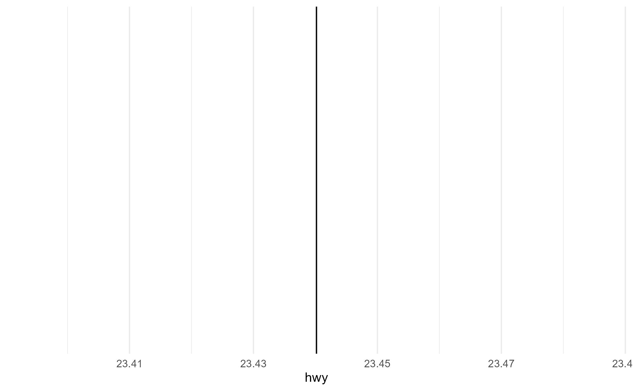

p2 + aes(fill = fl, color = drv)

Step 3.5 - Testing the solution

If you want to write tests, we can also check whether solution generalizes to other cases.

Here, we can see it correctly works with facets even when some groups are missing in a facet, so that’s good

p2 +
  aes(color = drv) +
  facet_wrap(~fl)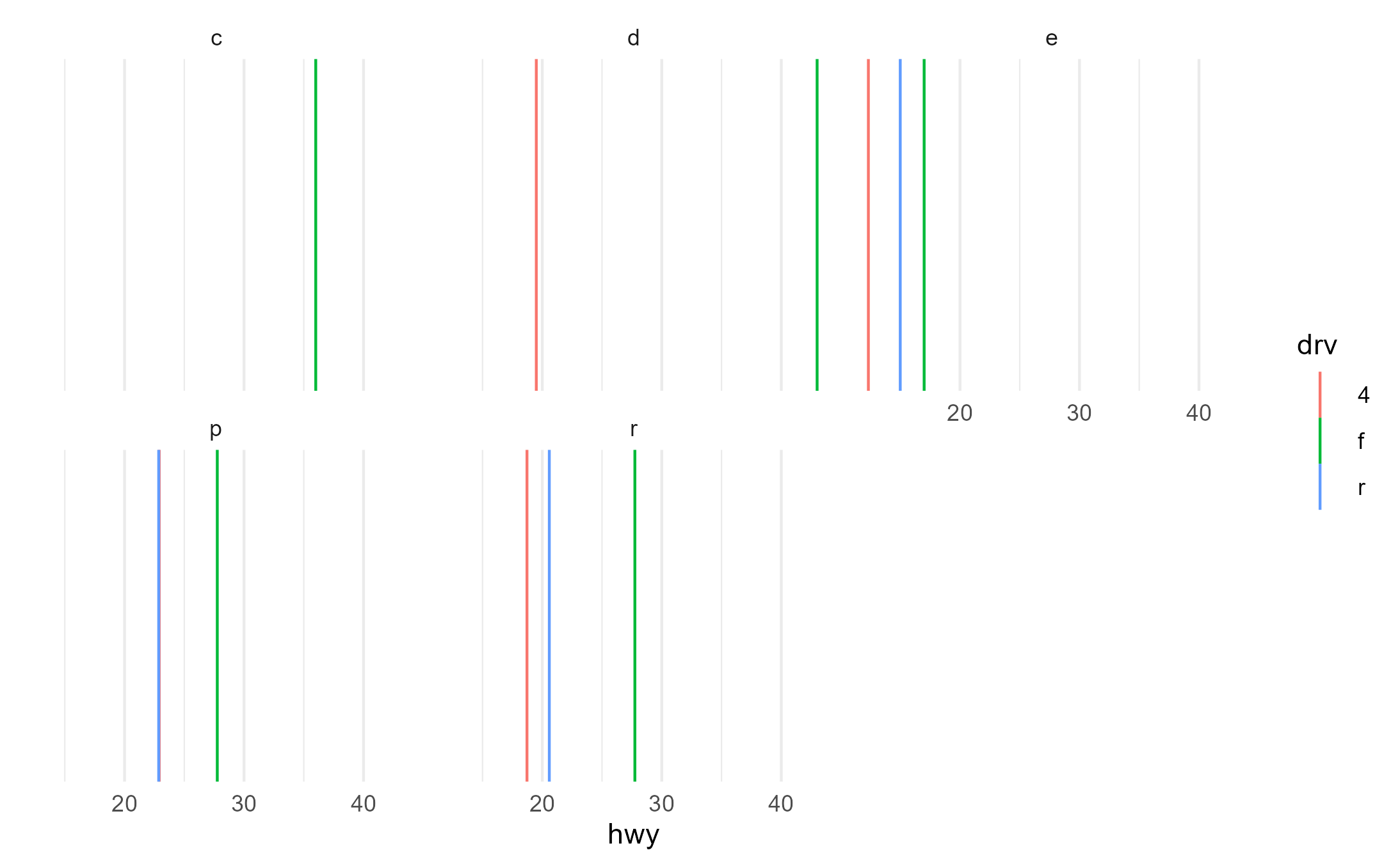

And we can also see that it fails the way it should when it’s supplied an explicit group aesthetic but also receives another discrete mapping to color

p2 + aes(group = fl, color = drv)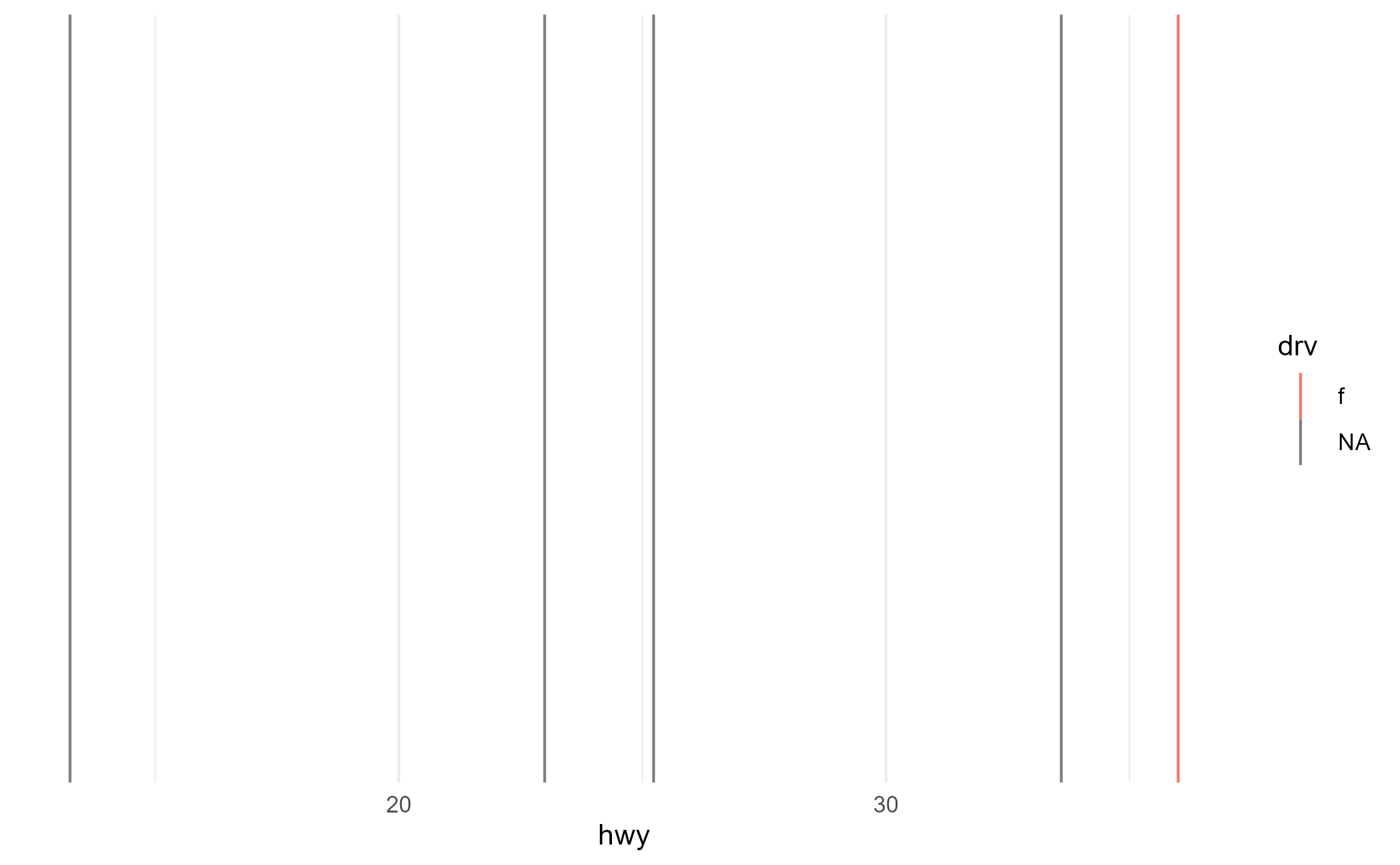

This is because there’s one unique match between fl == "c" and drv== "f", but no unique value for drv for the other four fl categories. So the color scale assigns a color to one of the lines but then for the other four lines it just gives up and returns NAs (which are colored grey by default)

table(mpg$drv, mpg$fl)
#>    
#>      c  d  e  p  r
#>   4  0  2  6 20 75
#>   f  1  3  1 25 76
#>   r  0  0  1  7 17
p2 +
  aes(group = fl, color = drv) +
  geom_label(aes(label = fl, y = 0), stat = StatXmean2)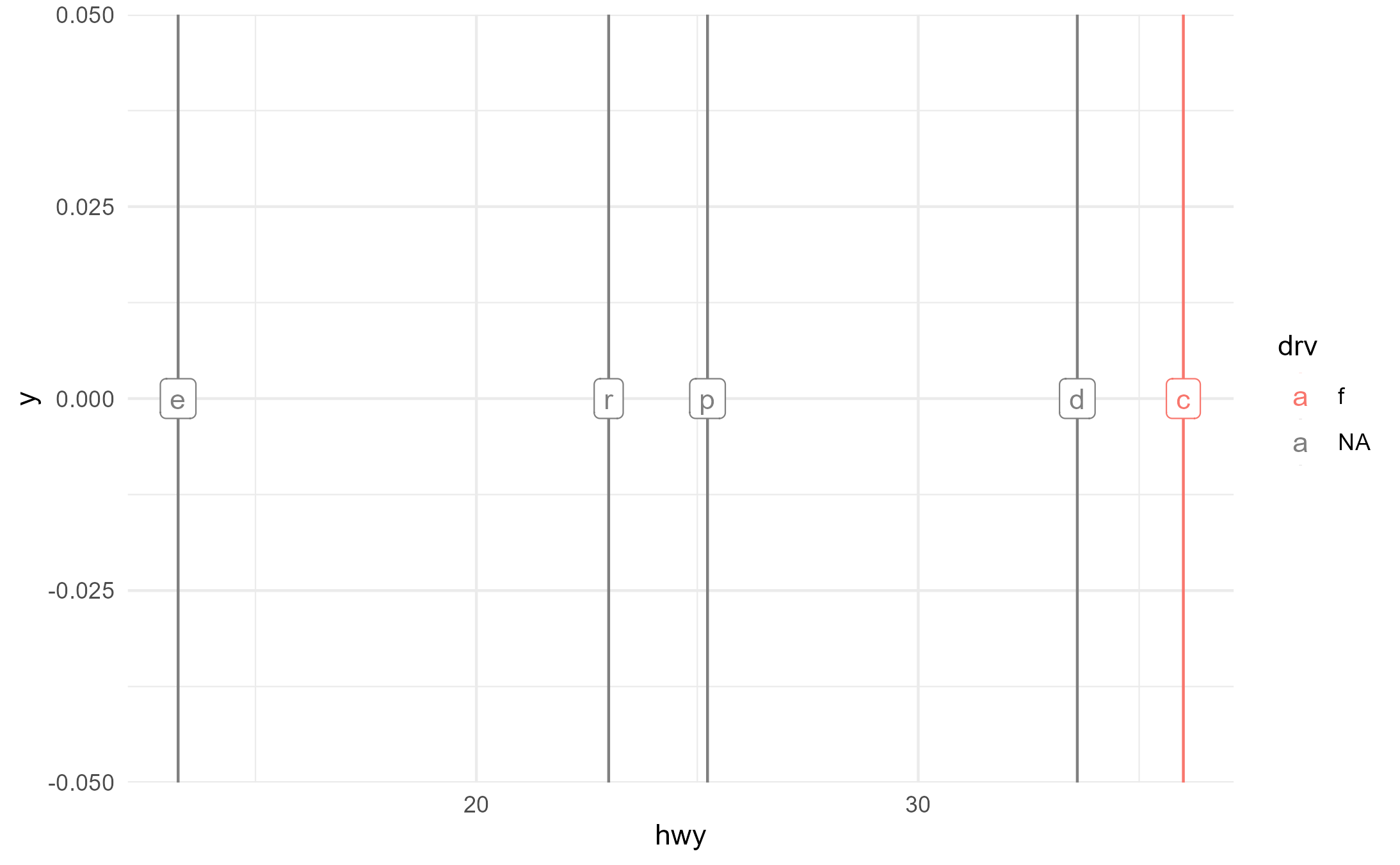

Wrapping up

We’re satisfied so we can now turn development mode off, which lets us access our current installation of {ggxmean} again. We can now also test our solution against the current version of the package to see whether it’d still work (although we skip that step here).

devtools::dev_mode(on = FALSE)
#> ✔ Dev mode: OFF
devtools::package_info("ggxmean", FALSE, FALSE)$source
#> [1] "local"

Finally, since this vignette covered a real-world debugging scenario, the solution has been submitted as a PR!

Many thanks to Gina for allowing me to use {ggxmean} as a case study for exploratory debugging with {ggtrace}!