In my last blogpost, I demonstrated a couple use cases for the higher-order functionals reduce() and accumulate() from the {purrr} package. In one example, I made an animated {kableExtra} table by accumulate()-ing over multiple calls to column_spec() that set a background color for a column.
Animated tables are virtually non-existent in the wild, and probably for a good reason. but I wanted to extend upon my previous table animation and create something that’s maybe a bit more on the “informative” side.
To that end, here’s an animate table that simulates sampling from a bivariate normal distribution.
Static
Let’s first start by generating 100,000 data points:
set.seed(2021)

library(dplyr)

samples_data <- MASS::mvrnorm(1e5, c(0, 0), matrix(c(1, .7, .7, 1), ncol = 2)) %>%
  as_tibble(.name_repair = ~c("x", "y")) %>%
  mutate(across(everything(), ~ as.character(.x - .x %% 0.2)))

samples_data
  # A tibble: 100,000 x 2
     x     y
     <chr> <chr>
   1 0     -0.4
   2 0.2   0.6
   3 0.4   0.2
   4 0.6   -0.2
   5 0.6   0.8
   6 -1.8  -2
   7 0.8   -0.6
   8 1.2   0.4
   9 0.4   -0.4
  10 1.4   1.6
  # ... with 99,990 more rows
Let’s see how this looks when we turn this into a “matrix”1. To place continuous values into discrete cells in the table, I’m also binning both variables by 0.2:
samples_data_spread <- samples_data %>%
  count(x, y) %>%
  right_join(
    tidyr::crossing(
      x = as.character(seq(-3, 3, 0.2)),
      y = as.character(seq(-3, 3, 0.2))
    ),
    by = c("x", "y")
  ) %>%
  tidyr::pivot_wider(names_from = y, values_from = n) %>%
  arrange(-as.numeric(x)) %>%
  select(c("x", as.character(seq(-3, 3, 0.2)))) %>%
  rename(" " = x)

samples_data_spread
  # A tibble: 31 x 32
     ` `    `-3` `-2.8` `-2.6` `-2.4` `-2.2`  `-2` `-1.8` `-1.6` `-1.4` `-1.2`
     <chr> <int>  <int>  <int>  <int>  <int> <int>  <int>  <int>  <int>  <int>
   1 3        NA     NA     NA     NA     NA    NA     NA     NA     NA     NA
   2 2.8      NA     NA     NA     NA     NA    NA     NA     NA     NA     NA
   3 2.6      NA     NA     NA     NA     NA    NA     NA     NA     NA     NA
   4 2.4      NA     NA     NA     NA     NA    NA     NA     NA     NA     NA
   5 2.2      NA     NA     NA     NA     NA    NA     NA     NA     NA     NA
   6 2        NA     NA     NA     NA     NA    NA     NA     NA     NA     NA
   7 1.8      NA     NA     NA     NA     NA    NA     NA     NA     NA     NA
   8 1.6      NA     NA     NA     NA     NA    NA     NA      1      1      4
   9 1.4      NA     NA     NA     NA     NA    NA      1     NA      1      4
  10 1.2      NA     NA     NA     NA     NA    NA     NA      3      2      7
  # ... with 21 more rows, and 21 more variables: `-1` <int>, `-0.8` <int>,
  #   `-0.6` <int>, `-0.4` <int>, `-0.2` <int>, `0` <int>, `0.2` <int>,
  #   `0.4` <int>, `0.6` <int>, `0.8` <int>, `1` <int>, `1.2` <int>, `1.4` <int>,
  #   `1.6` <int>, `1.8` <int>, `2` <int>, `2.2` <int>, `2.4` <int>, `2.6` <int>,
  #   `2.8` <int>, `3` <int>
Now we can turn this into a table and fill the cells according to the counts using reduce():
library(kableExtra)
samples_data_table <- samples_data_spread %>%
kable() %>%
kable_classic() %>%
purrr::reduce(2L:length(samples_data_spread), ~ {
column_spec(
kable_input = .x,
column = .y,
background = spec_color(
samples_data_spread[[.y]],
scale_from = c(1, max(as.numeric(as.matrix(samples_data_spread)), na.rm = TRUE)),
na_color = "white",
option = "plasma"
),
color = "white"
)},
.init = .
)
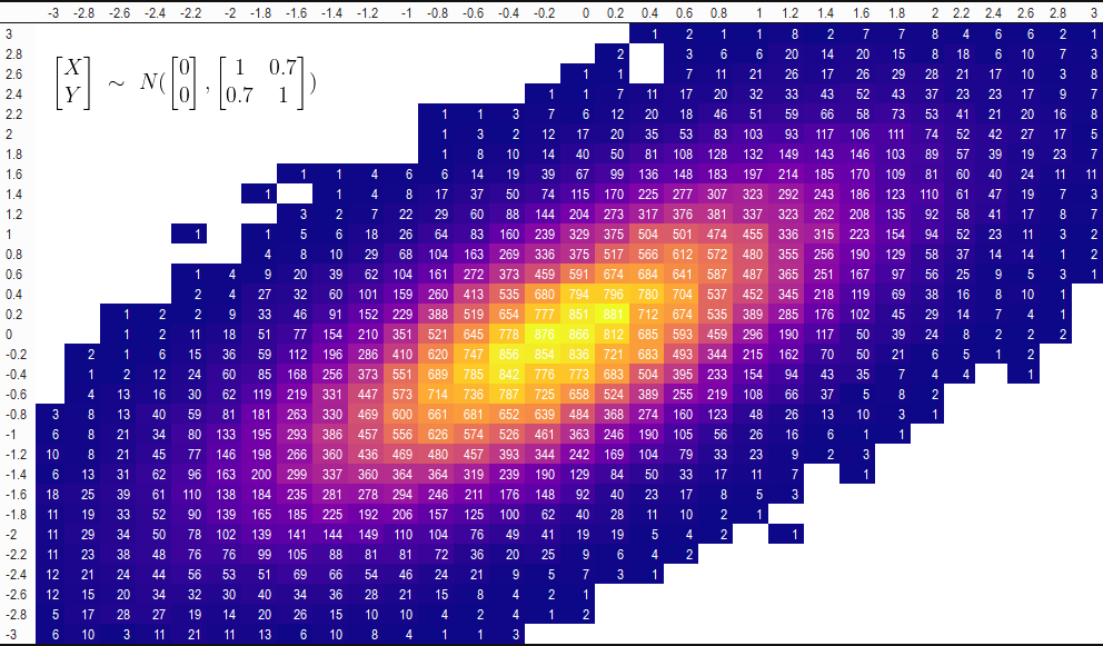
samples_data_table
| -3 | -2.8 | -2.6 | -2.4 | -2.2 | -2 | -1.8 | -1.6 | -1.4 | -1.2 | -1 | -0.8 | -0.6 | -0.4 | -0.2 | 0 | 0.2 | 0.4 | 0.6 | 0.8 | 1 | 1.2 | 1.4 | 1.6 | 1.8 | 2 | 2.2 | 2.4 | 2.6 | 2.8 | 3 | |
|---|---|---|---|---|---|---|---|---|---|---|---|---|---|---|---|---|---|---|---|---|---|---|---|---|---|---|---|---|---|---|---|
| 3 | NA | NA | NA | NA | NA | NA | NA | NA | NA | NA | NA | NA | NA | NA | NA | NA | NA | 1 | 2 | 1 | 1 | 8 | 2 | 7 | 7 | 8 | 4 | 6 | 6 | 2 | 1 |
| 2.8 | NA | NA | NA | NA | NA | NA | NA | NA | NA | NA | NA | NA | NA | NA | NA | NA | 2 | NA | 3 | 6 | 6 | 20 | 14 | 20 | 15 | 8 | 18 | 6 | 10 | 7 | 3 |
| 2.6 | NA | NA | NA | NA | NA | NA | NA | NA | NA | NA | NA | NA | NA | NA | NA | 1 | 1 | NA | 7 | 11 | 21 | 26 | 17 | 26 | 29 | 28 | 21 | 17 | 10 | 3 | 8 |
| 2.4 | NA | NA | NA | NA | NA | NA | NA | NA | NA | NA | NA | NA | NA | NA | 1 | 1 | 7 | 11 | 17 | 20 | 32 | 33 | 43 | 52 | 43 | 37 | 23 | 23 | 17 | 9 | 7 |
| 2.2 | NA | NA | NA | NA | NA | NA | NA | NA | NA | NA | NA | 1 | 1 | 3 | 7 | 6 | 12 | 20 | 18 | 46 | 51 | 59 | 66 | 58 | 73 | 53 | 41 | 21 | 20 | 16 | 8 |
| 2 | NA | NA | NA | NA | NA | NA | NA | NA | NA | NA | NA | 1 | 3 | 2 | 12 | 17 | 20 | 35 | 53 | 83 | 103 | 93 | 117 | 106 | 111 | 74 | 52 | 42 | 27 | 17 | 5 |
| 1.8 | NA | NA | NA | NA | NA | NA | NA | NA | NA | NA | NA | 1 | 8 | 10 | 14 | 40 | 50 | 81 | 108 | 128 | 132 | 149 | 143 | 146 | 103 | 89 | 57 | 39 | 19 | 23 | 7 |
| 1.6 | NA | NA | NA | NA | NA | NA | NA | 1 | 1 | 4 | 6 | 6 | 14 | 19 | 39 | 67 | 99 | 136 | 148 | 183 | 197 | 214 | 185 | 170 | 109 | 81 | 60 | 40 | 24 | 11 | 11 |
| 1.4 | NA | NA | NA | NA | NA | NA | 1 | NA | 1 | 4 | 8 | 17 | 37 | 50 | 74 | 115 | 170 | 225 | 277 | 307 | 323 | 292 | 243 | 186 | 123 | 110 | 61 | 47 | 19 | 7 | 3 |
| 1.2 | NA | NA | NA | NA | NA | NA | NA | 3 | 2 | 7 | 22 | 29 | 60 | 88 | 144 | 204 | 273 | 317 | 376 | 381 | 337 | 323 | 262 | 208 | 135 | 92 | 58 | 41 | 17 | 8 | 7 |
| 1 | NA | NA | NA | NA | 1 | NA | 1 | 5 | 6 | 18 | 26 | 64 | 83 | 160 | 239 | 329 | 375 | 504 | 501 | 474 | 455 | 336 | 315 | 223 | 154 | 94 | 52 | 23 | 11 | 3 | 2 |
| 0.8 | NA | NA | NA | NA | NA | NA | 4 | 8 | 10 | 29 | 68 | 104 | 163 | 269 | 336 | 375 | 517 | 566 | 612 | 572 | 480 | 355 | 256 | 190 | 129 | 58 | 37 | 14 | 14 | 1 | 2 |
| 0.6 | NA | NA | NA | NA | 1 | 4 | 9 | 20 | 39 | 62 | 104 | 161 | 272 | 373 | 459 | 591 | 674 | 684 | 641 | 587 | 487 | 365 | 251 | 167 | 97 | 56 | 25 | 9 | 5 | 3 | 1 |
| 0.4 | NA | NA | NA | NA | 2 | 4 | 27 | 32 | 60 | 101 | 159 | 260 | 413 | 535 | 680 | 794 | 796 | 780 | 704 | 537 | 452 | 345 | 218 | 119 | 69 | 38 | 16 | 8 | 10 | 1 | NA |
| 0.2 | NA | NA | 1 | 2 | 2 | 9 | 33 | 46 | 91 | 152 | 229 | 388 | 519 | 654 | 777 | 851 | 881 | 712 | 674 | 535 | 389 | 285 | 176 | 102 | 45 | 29 | 14 | 7 | 4 | 1 | NA |
| 0 | NA | NA | 1 | 2 | 11 | 18 | 51 | 77 | 154 | 210 | 351 | 521 | 645 | 778 | 876 | 866 | 812 | 685 | 593 | 459 | 296 | 190 | 117 | 50 | 39 | 24 | 8 | 2 | 2 | 2 | NA |
| -0.2 | NA | 2 | 1 | 6 | 15 | 36 | 59 | 112 | 196 | 286 | 410 | 620 | 747 | 856 | 854 | 836 | 721 | 683 | 493 | 344 | 215 | 162 | 70 | 50 | 21 | 6 | 5 | 1 | 2 | NA | NA |
| -0.4 | NA | 1 | 2 | 12 | 24 | 60 | 85 | 168 | 256 | 373 | 551 | 689 | 785 | 842 | 776 | 773 | 683 | 504 | 395 | 233 | 154 | 94 | 43 | 35 | 7 | 4 | 4 | NA | 1 | NA | NA |
| -0.6 | NA | 4 | 13 | 16 | 30 | 62 | 119 | 219 | 331 | 447 | 573 | 714 | 736 | 787 | 725 | 658 | 524 | 389 | 255 | 219 | 108 | 66 | 37 | 5 | 8 | 2 | NA | NA | NA | NA | NA |
| -0.8 | 3 | 8 | 13 | 40 | 59 | 81 | 181 | 263 | 330 | 469 | 600 | 661 | 681 | 652 | 639 | 484 | 368 | 274 | 160 | 123 | 48 | 26 | 13 | 10 | 3 | 1 | NA | NA | NA | NA | NA |
| -1 | 6 | 8 | 21 | 34 | 80 | 133 | 195 | 293 | 386 | 457 | 556 | 626 | 574 | 526 | 461 | 363 | 246 | 190 | 105 | 56 | 26 | 16 | 6 | 1 | 1 | NA | NA | NA | NA | NA | NA |
| -1.2 | 10 | 8 | 21 | 45 | 77 | 146 | 198 | 266 | 360 | 436 | 469 | 480 | 457 | 393 | 344 | 242 | 169 | 104 | 79 | 33 | 23 | 9 | 2 | 3 | NA | NA | NA | NA | NA | NA | NA |
| -1.4 | 6 | 13 | 31 | 62 | 96 | 163 | 200 | 299 | 337 | 360 | 364 | 364 | 319 | 239 | 190 | 129 | 84 | 50 | 33 | 17 | 11 | 7 | NA | 1 | NA | NA | NA | NA | NA | NA | NA |
| -1.6 | 18 | 25 | 39 | 61 | 110 | 138 | 184 | 235 | 281 | 278 | 294 | 246 | 211 | 176 | 148 | 92 | 40 | 23 | 17 | 8 | 5 | 3 | NA | NA | NA | NA | NA | NA | NA | NA | NA |
| -1.8 | 11 | 19 | 33 | 52 | 90 | 139 | 165 | 185 | 225 | 192 | 206 | 157 | 125 | 100 | 62 | 40 | 28 | 11 | 10 | 2 | 1 | NA | NA | NA | NA | NA | NA | NA | NA | NA | NA |
| -2 | 11 | 29 | 34 | 50 | 78 | 102 | 139 | 141 | 144 | 149 | 110 | 104 | 76 | 49 | 41 | 19 | 19 | 5 | 4 | 2 | NA | 1 | NA | NA | NA | NA | NA | NA | NA | NA | NA |
| -2.2 | 11 | 23 | 38 | 48 | 76 | 76 | 99 | 105 | 88 | 81 | 81 | 72 | 36 | 20 | 25 | 9 | 6 | 4 | 2 | NA | NA | NA | NA | NA | NA | NA | NA | NA | NA | NA | NA |
| -2.4 | 12 | 21 | 24 | 44 | 56 | 53 | 51 | 69 | 66 | 54 | 46 | 24 | 21 | 9 | 5 | 7 | 3 | 1 | NA | NA | NA | NA | NA | NA | NA | NA | NA | NA | NA | NA | NA |
| -2.6 | 12 | 15 | 20 | 34 | 32 | 30 | 40 | 34 | 36 | 28 | 21 | 15 | 8 | 4 | 2 | 1 | NA | NA | NA | NA | NA | NA | NA | NA | NA | NA | NA | NA | NA | NA | NA |
| -2.8 | 5 | 17 | 28 | 27 | 19 | 14 | 20 | 26 | 15 | 10 | 10 | 4 | 2 | 4 | 1 | 2 | NA | NA | NA | NA | NA | NA | NA | NA | NA | NA | NA | NA | NA | NA | NA |
| -3 | 6 | 10 | 3 | 11 | 21 | 11 | 13 | 6 | 10 | 8 | 4 | 1 | 1 | 3 | NA | NA | NA | NA | NA | NA | NA | NA | NA | NA | NA | NA | NA | NA | NA | NA | NA |
An aside on LaTeX equations
As an aside, let’s say we also want to annotate this table with the true distribution where this sample came from. As specified in our call to MASS::mvrnorm() used to make samples_data, the distribution is one where both variables have a mean of 0 and a standard deviation of 1, plus a correlation of 0.7:
\[\begin{bmatrix} X \\ Y \end{bmatrix}\ \sim\ N(\begin{bmatrix} 0 \\ 0 \end{bmatrix},\begin{bmatrix}1 & 0.7 \\ 0.7 & 1 \end{bmatrix})\]
Where the LaTeX code for the above formula is:
  \begin{bmatrix} X \\ Y \end{bmatrix}\ \sim\
  N(\begin{bmatrix} 0 \\ 0 \end{bmatrix},
  \begin{bmatrix}1 & 0.7 \\ 0.7 & 1 \end{bmatrix})
Many different solutions already exist to LaTeX math annotations. The most common is probably Non-Standard Evaluation (NSE) methods using parse(), expression(), bquote() etc. There are bulkier solutions like the {latex2exp} package that plots plotmath expressions, though it hasn’t been updated since 2015 and I personally had difficulty getting it to work.
One solution I’ve never heard of/considered before is querying a web LaTeX editor that has an API. The Online LaTeX Equation Editor by CodeCogs is the perfect example of this. A simple link that contains the LaTeX code in a URL-compatible encoding renders the resulting expression as an image!
I wrote a function latex_query (not thoroughly tested) in my personal package that takes LaTeX code and generates a CodeCogs URL containing the rendered expression2
# NOTE the string literal syntax using r"(...)" is only available in R 4.0.0 and up
latex_url <- junebug::latex_query(
  formula = r"(\begin{bmatrix} X \\ Y \end{bmatrix}\ \sim\
              N(\begin{bmatrix} 0 \\ 0 \end{bmatrix},
              \begin{bmatrix}1 & 0.7 \\ 0.7 & 1 \end{bmatrix}))",
  dpi = 150
)

knitr::include_graphics(latex_url)
The variable latex_url is this really long URL which, as we see above, points to a rendered image of the LaTeX expression we fed it!
Annotating our table, then, is pretty straightforward. We save it as an image, read in the LaTeX equation as an image, then combine!
save_kable(samples_data_table, "img/samples_data_table.png")

library(magick)

image_composite(
  image_read("img/samples_data_table.png"),
  image_read(latex_url),
  offset = "+50+50"
)
Animated
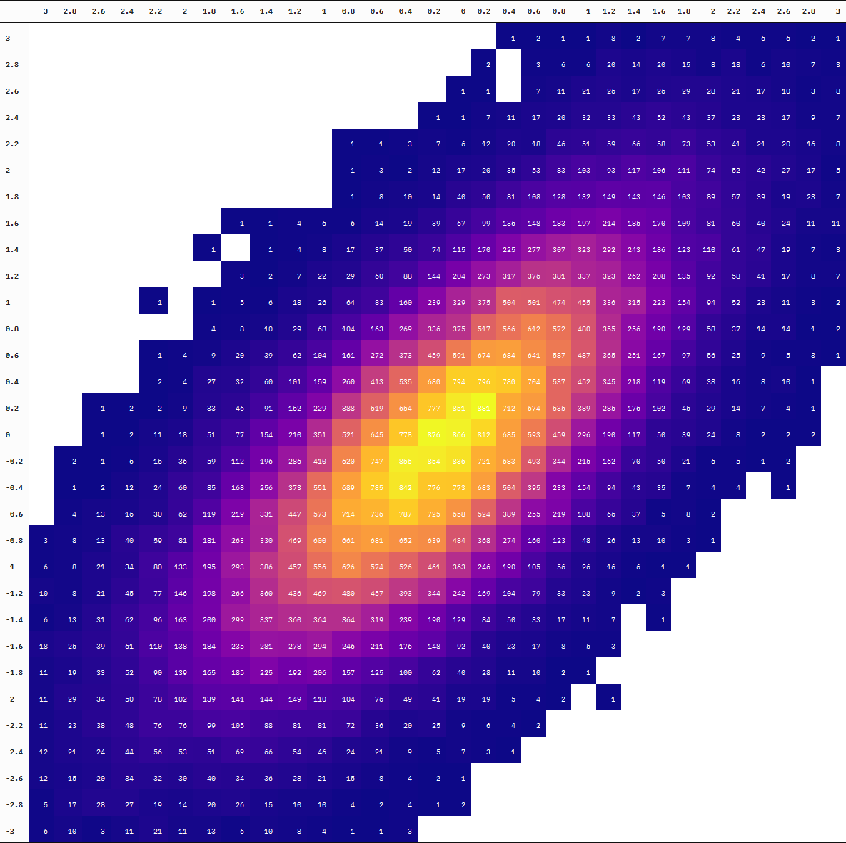
For an animated version, we add a step where we split the data at every 10,000 additional samples before binning the observations into cells. We then draw a table at each point of the accumulation using {kableExtra} with the help of map() and reduce() (plus some more kable styling).
samples_tables <- purrr::map(1L:10L, ~{
  samples_slice <- samples_data %>%
    slice(1L:(.x * 1e4)) %>%
    count(x, y) %>%
    right_join(
      tidyr::crossing(
        x = as.character(seq(-3, 3, 0.2)),
        y = as.character(seq(-3, 3, 0.2))
      ),
      by = c("x", "y")
    ) %>%
    tidyr::pivot_wider(names_from = y, values_from = n) %>%
    arrange(-as.numeric(x)) %>%
    select(c("x", as.character(seq(-3, 3, 0.2)))) %>%
    rename(" " = x)


  samples_slice %>%
    kable() %>%
    kable_classic() %>%
    purrr::reduce(
      2L:length(samples_slice),
      ~ {
        .x %>%
          column_spec(
            column = .y,
            width_min = "35px",
            background = spec_color(
              samples_slice[[.y]],
              scale_from = c(1, max(as.numeric(as.matrix(samples_slice)), na.rm = TRUE)),
              na_color = "white",
              option = "plasma"
            ),
            color = "white"
          ) %>%
          row_spec(
            row = .y - 1L,
            hline_after = FALSE,
            extra_css = "border-top:none; padding-top:15px;"
          )
      },
      .init = .
    ) %>%
    row_spec(0L, bold = TRUE) %>%
    column_spec(1L, bold = TRUE, border_right = TRUE) %>%
    kable_styling(
      full_width = F,
      font_size = 10,
      html_font = "IBM Plex Mono",
    )
})
The result, samples_tables is a list of tables. We can walk() over that list with save_kable() to write them as images and then read them back in with {magick}:
purrr::iwalk(samples_tables, ~ save_kable(.x, file = glue::glue("tbl_imgs/tbl{.y}.png")))

table_imgs <- image_read(paste0("tbl_imgs/tbl", 1:10, ".png"))
Now we can add our LaTeX expression from the previous section as an annotation to these table images using image_composite():
table_imgs_annotated <- table_imgs %>%
  image_composite(
    image_read(latex_url),
    offset = "+100+80"
  )
Finally, we just patch the table images together into an animation using image_animate() and we have our animated table!
table_imgs_animated <- table_imgs_annotated %>%
  image_animate(optimize = TRUE)
Final Product
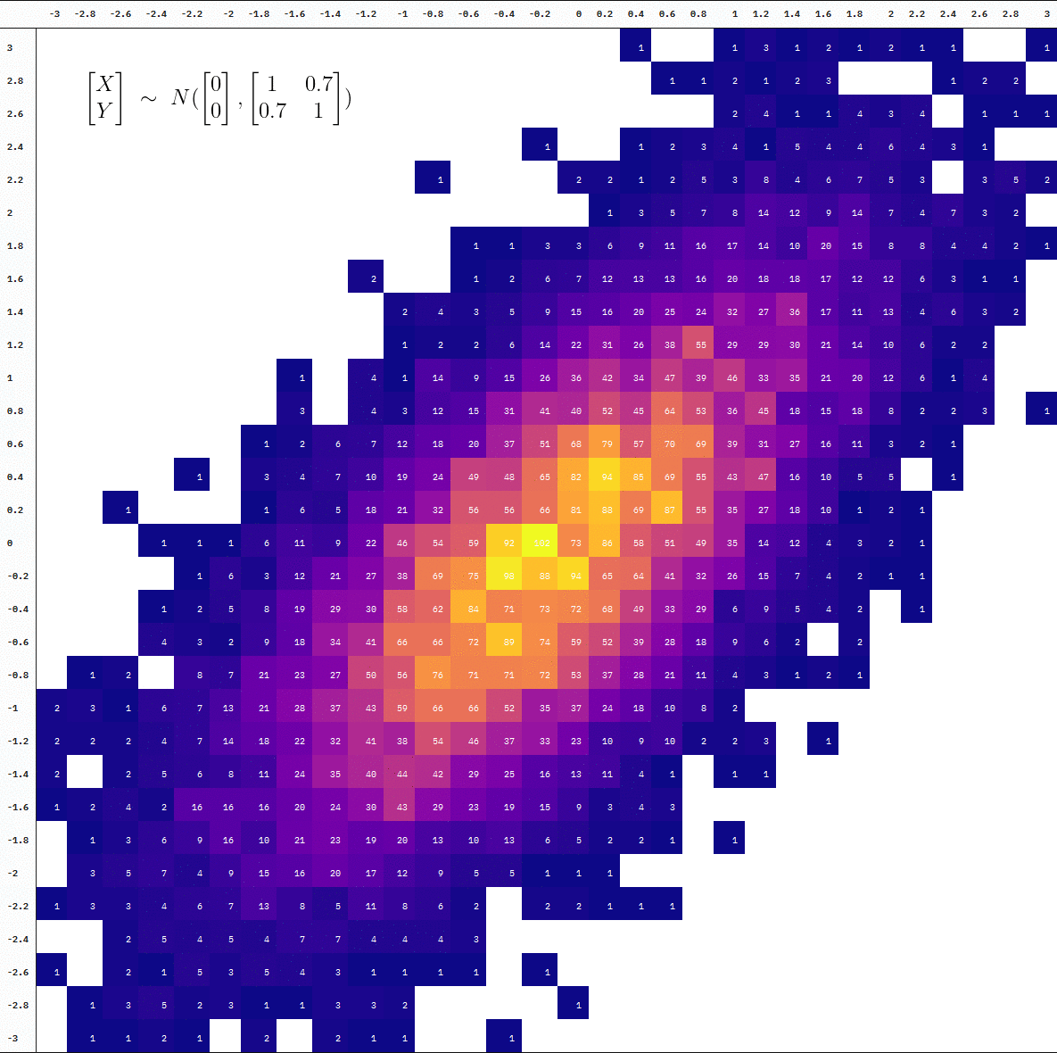
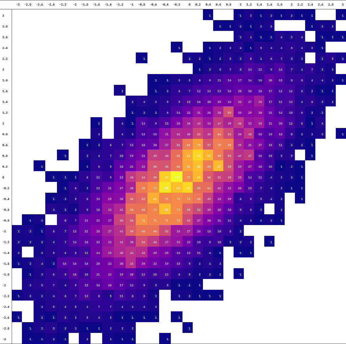
You can also see the difference in the degree of “interpolation” by directly comparing the table at 10 thousand vs 100 thousand samples (the first and last frames):
Neat!
Visually speaking. It’s still a dataframe object for compatibility with {kableExtra}↩︎
Details about the API - https://www.codecogs.com/latex/editor-api.php↩︎