Introduction
Happy pipes
Modern day programming with R is all about pipes.1 You start out with some object that undergoes incremental changes as it is passed (piped) into a chain of functions and finally returned as the desired output, like in this simple example. 2
set.seed(2021) # Can 2020 be over already?

square <- function(x) x^2
deviation <- function(x) x - mean(x)

nums <- runif(100)

nums %>%
  deviation() %>%
  square() %>%
  mean() %>%
  sqrt()
[1] 0.3039881When we pipe (or pass anything through any function, for that matter), we often do one distinct thing at a time, like in the above example.
So, we rarely have a chain of functions that look like this:
… because many functions are vectorized, or designed to handle multiple values by other means, like this:
Sad (repetitive) pipes
But some functions do not handle multiple inputs the way we want it to, or just not at all. Here are some examples of what I’m talking about.
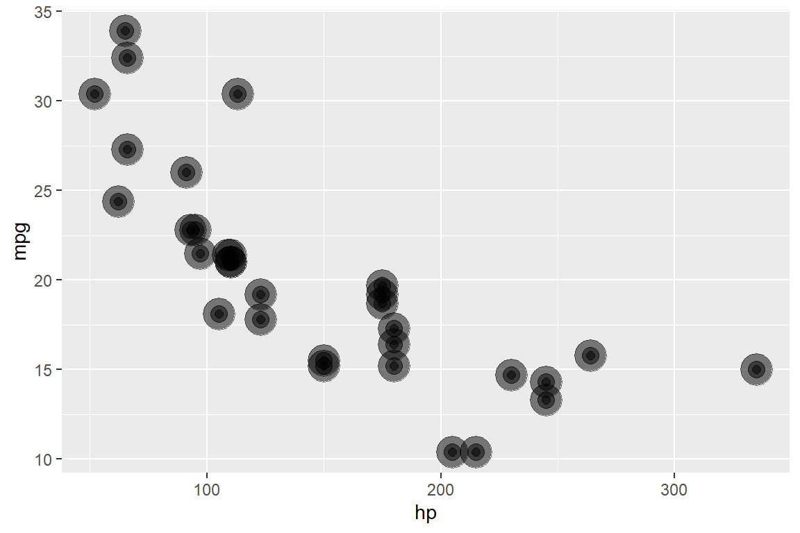
In {ggplot2}, this doesn’t plot 3 overlapping points with sizes 8, 4, and 2:
Error: Aesthetics must be either length 1 or the same as the data (32): sizeSo you have to do this:
ggplot(mtcars, aes(hp, mpg)) +
  geom_point(size = 8, alpha = .5) +
  geom_point(size = 4, alpha = .5) +
  geom_point(size = 2, alpha = .5)

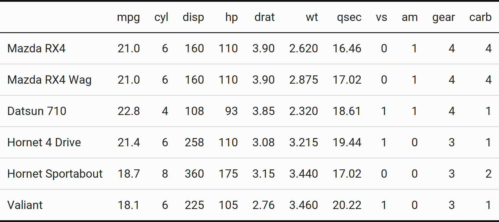
In {kableExtra}, this doesn’t color the third column “skyblue”, the fourth column “forestgreen”, and the fifth column “chocolate”:3
library(kableExtra)

mtcars %>%
  head() %>%
  kbl() %>%
  kable_classic(html_font = "Roboto") %>%
  column_spec(3:5, background = c("skyblue", "forestgreen", "chocolate"))
  Warning in ensure_len_html(background, nrows, "background"): The number of
provided values in background does not equal to the number of rows.| mpg | cyl | disp | hp | drat | wt | qsec | vs | am | gear | carb | |
|---|---|---|---|---|---|---|---|---|---|---|---|
| Mazda RX4 | 21.0 | 6 | 160 | 110 | 3.90 | 2.620 | 16.46 | 0 | 1 | 4 | 4 |
| Mazda RX4 Wag | 21.0 | 6 | 160 | 110 | 3.90 | 2.875 | 17.02 | 0 | 1 | 4 | 4 |
| Datsun 710 | 22.8 | 4 | 108 | 93 | 3.85 | 2.320 | 18.61 | 1 | 1 | 4 | 1 |
| Hornet 4 Drive | 21.4 | 6 | 258 | 110 | 3.08 | 3.215 | 19.44 | 1 | 0 | 3 | 1 |
| Hornet Sportabout | 18.7 | 8 | 360 | 175 | 3.15 | 3.440 | 17.02 | 0 | 0 | 3 | 2 |
| Valiant | 18.1 | 6 | 225 | 105 | 2.76 | 3.460 | 20.22 | 1 | 0 | 3 | 1 |
So you have to do this:
mtcars %>%
  head() %>%
  kbl() %>%
  kable_classic(html_font = "Roboto") %>%
  column_spec(3, background = "skyblue") %>%
  column_spec(4, background = "forestgreen") %>%
  column_spec(5, background = "chocolate")
| mpg | cyl | disp | hp | drat | wt | qsec | vs | am | gear | carb | |
|---|---|---|---|---|---|---|---|---|---|---|---|
| Mazda RX4 | 21.0 | 6 | 160 | 110 | 3.90 | 2.620 | 16.46 | 0 | 1 | 4 | 4 |
| Mazda RX4 Wag | 21.0 | 6 | 160 | 110 | 3.90 | 2.875 | 17.02 | 0 | 1 | 4 | 4 |
| Datsun 710 | 22.8 | 4 | 108 | 93 | 3.85 | 2.320 | 18.61 | 1 | 1 | 4 | 1 |
| Hornet 4 Drive | 21.4 | 6 | 258 | 110 | 3.08 | 3.215 | 19.44 | 1 | 0 | 3 | 1 |
| Hornet Sportabout | 18.7 | 8 | 360 | 175 | 3.15 | 3.440 | 17.02 | 0 | 0 | 3 | 2 |
| Valiant | 18.1 | 6 | 225 | 105 | 2.76 | 3.460 | 20.22 | 1 | 0 | 3 | 1 |
In {dplyr}, this doesn’t make 3 new columns named “a”, “b”, and “c”, all filled with NA:4
Error: The LHS of `:=` must be a string or a symbolSo you have to do either one of these:5
     mpg  a  b  c
  1 21.0 NA NA NA
  2 21.0 NA NA NA
  3 22.8 NA NA NA
  4 21.4 NA NA NA
  5 18.7 NA NA NA
  6 18.1 NA NA NA
So we’ve got functions being repeated, but in all these cases it looks like we can’t just throw in a vector and expect the function to loop/map over them internally in the specific way that we want it to. And the “correct ways” I provided here are not very satisfying: that’s a lot of copying and pasting!
Personally, I think it’d be nice to collapse these repetitive calls - but how?
Introducing purrr::reduce()
The reduce() function from the {purrr} package is a powerful functional that allows you to abstract away from a sequence of functions that are applied in a fixed direction. You should go give Advanced R Ch. 9.5 a read if you want an in-depth explanation, but here I’m just gonna give a quick crash course for our application of it to our current problem.6
All you need to know here is that reduce() takes a vector as its first argument, a function as its second argument, and an optional .init argument.7
Here’s a schematic:
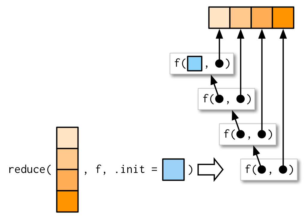
Figure 1: From Advanced R by Hadley Wickham
Let me really quickly demonstrate reduce() in action.
Say you wanted to add up the numbers 1 through 5, but only using the plus operator +. You could do something like this:8
1 + 2 + 3 + 4 + 5
[1] 15Which is the same as this:
And if you want the start value to be something that’s not the first argument of the vector, pass that to the .init argument:
If you want to be specific, you can use an {rlang}-style anonymous function where .x is the accumulated value being passed into the first argument fo the function and .y is the second argument of the function.9
And two more examples just to demonstrate that directionality matters:
identical(
  reduce(1:5, `^`, .init = 0.5),
  reduce(1:5, ~ .x ^ .y, .init = 0.5) # .x on left, .y on right
)
[1] TRUEidentical(
reduce(1:5, `^`, .init = 0.5),
reduce(1:5, ~ .y ^ .x, .init = 0.5) # .y on left, .x on right
)
[1] FALSEThat’s pretty much all you need to know - let’s jump right in!
Example 1: {ggplot2}
A reduce() solution
Recall that we had this sad code:
ggplot(mtcars, aes(hp, mpg)) +
  geom_point(size = 8, alpha = .5) +
  geom_point(size = 4, alpha = .5) +
  geom_point(size = 2, alpha = .5)
For illustrative purposes, I’m going to move the + “pipes” to the beginning of each line:
ggplot(mtcars, aes(hp, mpg))
  + geom_point(size = 8, alpha = .5)
  + geom_point(size = 4, alpha = .5)
  + geom_point(size = 2, alpha = .5)
At this point, we see a clear pattern emerge line-by-line. We start with ggplot(mtcars, aes(hp, mpg)), which is kind of its own thing. Then we have three repetitions of + geom_point(size = X, alpha = .5) where the X varies between 8, 4, and 2. We also notice that the sequence of calls goes from left to right, as is the normal order of piping.
Now let’s translate these observations into reduce(). I’m bad with words so here’s a visual:
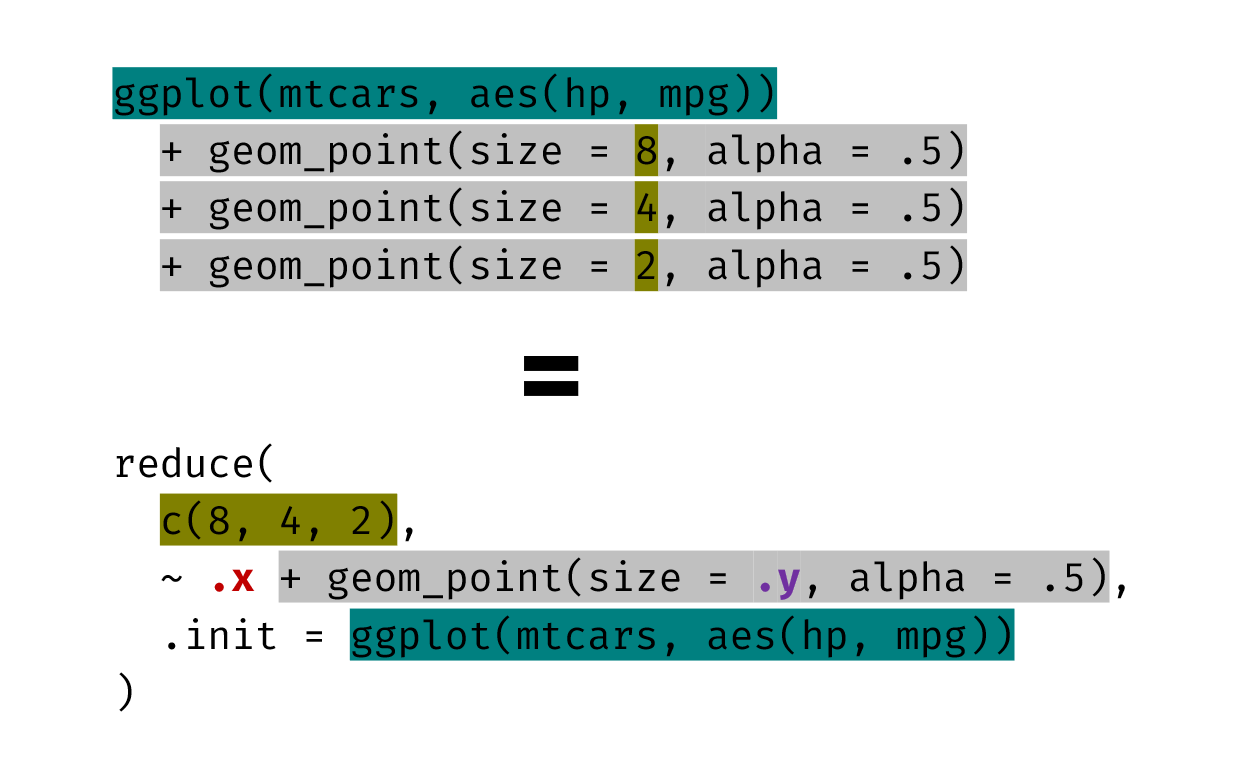
Let’s go over what we did in our call to reduce() above:
In the first argument, we have the vector of values that are iterated over.
In the second argument, we have an anonymous function composed of…
The
.xvariable, which represents the accumulated value. In this context, we keep the.xon the left because that is the left-hand side that we are carrying over to the next call via the+.The
.yvariable, which takes on values from the first argument passed intoreduce(). In this context,.ywill be each value of the numeric vectorc(8, 4, 2)since.initis given.The repeating function call
geom_point(size = .y, alpha = .5)that is called with each value of the vector passed in as the first argument.
In the third argument
.init, we haveggplot(mtcars, aes(hp, mpg))which is the non-repeating piece of code that we start with.
If you want to see the actual code run, here it is:
reduce(
  c(8, 4, 2),
  ~ .x + geom_point(size = .y, alpha = .5),
  .init = ggplot(mtcars, aes(hp, mpg))
)
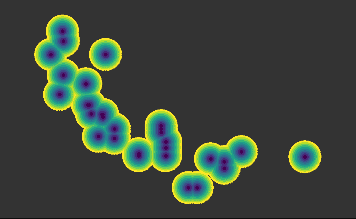
Let’s dig in a bit more, this time with an example that looks prettier.
Suppose you want to collapse the repeated calls to geom_point() in this code:
viridis_colors <- viridis::viridis(10)

mtcars %>%
  ggplot(aes(hp, mpg)) +
  geom_point(size = 20, color = viridis_colors[10]) +
  geom_point(size = 18, color = viridis_colors[9]) +
  geom_point(size = 16, color = viridis_colors[8]) +
  geom_point(size = 14, color = viridis_colors[7]) +
  geom_point(size = 12, color = viridis_colors[6]) +
  geom_point(size = 10, color = viridis_colors[5]) +
  geom_point(size = 8, color = viridis_colors[4]) +
  geom_point(size = 6, color = viridis_colors[3]) +
  geom_point(size = 4, color = viridis_colors[2]) +
  geom_point(size = 2, color = viridis_colors[1]) +
  scale_x_discrete(expand = expansion(.2)) +
  scale_y_continuous(expand = expansion(.2)) +
  theme_void() +
  theme(panel.background = element_rect(fill = "grey20"))
You can do this with reduce() in a couple ways:10
Method 1
Method 1: Move all the “constant” parts to .init, since the order of these layers don’t matter.
reduce(
    10L:1L,
    ~ .x + geom_point(size = .y * 2, color = viridis_colors[.y]),

    .init = mtcars %>%
      ggplot(aes(hp, mpg)) +
      scale_x_discrete(expand = expansion(.2)) +
      scale_y_continuous(expand = expansion(.2)) +
      theme_void() +
      theme(panel.background = element_rect(fill = "grey20"))

)
Method 2
Method 2: Use reduce() in place, with the help of the {magrittr} dot .
mtcars %>%
  ggplot(aes(hp, mpg)) %>%

  reduce(
    10L:1L,
    ~ .x + geom_point(size = .y * 2, color = viridis_colors[.y]),
    .init = . #<- right here!
  ) +

  scale_x_discrete(expand = expansion(.2)) +
  scale_y_continuous(expand = expansion(.2)) +
  theme_void() +
  theme(panel.background = element_rect(fill = "grey20"))
Method 3
Method 3: Move all the “constant” parts to the top, wrap it in parentheses, and pass the whole thing into .init using the {magrittr} dot .
(mtcars %>%
  ggplot(aes(hp, mpg)) +
  scale_x_discrete(expand = expansion(.2)) +
  scale_y_continuous(expand = expansion(.2)) +
  theme_void() +
  theme(panel.background = element_rect(fill = "grey20"))) %>%

  reduce(
    10L:1L,
    ~ .x + geom_point(size = .y * 2, color = viridis_colors[.y]),
    .init = . #<- right here!
  )
All in all, we see that reduce() allows us to write more succinct code!
An obvious advantage to this is that it is now really easy to make a single change that applies to all the repeated calls.
For example, if I want to make the radius of the points grow/shrink exponentially, I just need to modify the anonymous function in the second argument of reduce():
# Using Method 3
(mtcars %>%
  ggplot(aes(hp, mpg)) +
  scale_x_discrete(expand = expansion(.2)) +
  scale_y_continuous(expand = expansion(.2)) +
  theme_void() +
  theme(panel.background = element_rect(fill = "grey20"))) %>%
  reduce(
    10L:1L,
    ~ .x + geom_point(size = .y ^ 1.5, color = viridis_colors[.y]),  # exponential!
    .init = .
  )
Yay, we collapsed ten layers of geom_point()!
feat. accumulate()
There’s actually one more thing I want to show here, which is holding onto intermediate values using accumulate().
accumulate() is like reduce(), except instead of returning a single value which is the output of the very last function call, it keeps all intermediate values and returns them in a list.
accumulate(1:5, `+`)
[1] 1 3 6 10 15Check out what happens if I change reduce() to accumulate() and return each element of the resulting list:
plots <- (mtcars %>%
  ggplot(aes(hp, mpg)) +
  scale_x_discrete(expand = expansion(.2)) +
  scale_y_continuous(expand = expansion(.2)) +
  theme_void() +
  theme(panel.background = element_rect(fill = "grey20"))) %>%
  accumulate(
    10L:1L,
    ~ .x + geom_point(size = .y ^ 1.5, color = viridis_colors[.y]),
    .init = .
  )

for (i in plots) { plot(i) }


We got back the intermediate plots!
Are you thinking what I’m thinking? Let’s animate this!
library(magick)

# change ggplot2 objects into images
imgs <- map(1:length(plots), ~ {
  img <- image_graph(width = 672, height = 480)
  plot(plots[[.x]])
  dev.off()
  img
})

# combine images as frames
imgs <- image_join(imgs)

# animate
image_animate(imgs)

Neat!11
Example 2: {kableExtra}
A reduce2() solution
Recall that we had this sad code:
mtcars %>%
  head() %>%
  kbl() %>%
  kable_classic(html_font = "Roboto") %>%
  column_spec(3, background = "skyblue") %>%
  column_spec(4, background = "forestgreen") %>%
  column_spec(5, background = "chocolate")
We’ve got two things varying here: the column location 3:5 and the background color c("skyblue", "forestgreen", "chocolate"). We could do the same trick I sneaked into the previous section by just passing one vector to reduce() that basically functions as an index:12
numbers <- 3:5
background_colors <- c("skyblue", "forestgreen", "chocolate")

(mtcars %>%
  head() %>%
  kbl() %>%
  kable_classic(html_font = "Roboto")) %>%
  reduce(
    1:3,
    ~ .x %>% column_spec(numbers[.y], background = background_colors[.y]),
    .init = .
  )
But I want to use this opportunity to showcase reduce2(), which explicitly takes a second varying argument to the function that you are reduce()-ing over.
Here, ..1 is like the .x and ..2 is like the .y from reduce(). The only new part is ..3 which refers to the second varying argument.
(mtcars %>%
  head() %>%
  kbl() %>%
  kable_classic(html_font = "Roboto")) %>%
  reduce2(
    3:5,                                           # 1st varying argument (represented by ..2)
    c("skyblue", "forestgreen", "chocolate"),      # 2nd varying argument (represented by ..3)
    ~ ..1 %>% column_spec(..2, background = ..3),
    .init = .
  )
We’re not done yet! We can actually skip the {magrittr} pipe %>% and just stick ..1 as the first argument inside column_spec().13 This actually improves performance because you’re removing the overhead from evaluating the pipe!
Additionally, because the pipe forces evaluation with each call unlike + in {ggplot2}, we don’t need the parantheses wrapped around the top part of the code for the {magrittr} dot . to work!
Here is the final reduce2() solution for our sad code:
mtcars %>%
  head() %>%
  kbl() %>%
  kable_classic(html_font = "Roboto") %>%       # No need to wrap in parentheses!
  reduce2(
    3:5,
    c("skyblue", "forestgreen", "chocolate"),
    ~ column_spec(..1, ..2, background = ..3),  # No need for the pipe!
    .init = .
  )
| mpg | cyl | disp | hp | drat | wt | qsec | vs | am | gear | carb | |
|---|---|---|---|---|---|---|---|---|---|---|---|
| Mazda RX4 | 21.0 | 6 | 160 | 110 | 3.90 | 2.620 | 16.46 | 0 | 1 | 4 | 4 |
| Mazda RX4 Wag | 21.0 | 6 | 160 | 110 | 3.90 | 2.875 | 17.02 | 0 | 1 | 4 | 4 |
| Datsun 710 | 22.8 | 4 | 108 | 93 | 3.85 | 2.320 | 18.61 | 1 | 1 | 4 | 1 |
| Hornet 4 Drive | 21.4 | 6 | 258 | 110 | 3.08 | 3.215 | 19.44 | 1 | 0 | 3 | 1 |
| Hornet Sportabout | 18.7 | 8 | 360 | 175 | 3.15 | 3.440 | 17.02 | 0 | 0 | 3 | 2 |
| Valiant | 18.1 | 6 | 225 | 105 | 2.76 | 3.460 | 20.22 | 1 | 0 | 3 | 1 |
And of course, we now have the flexibilty to do much more complicated manipulations!
mtcars %>%
  head() %>%
  kbl() %>%
  kable_classic(html_font = "Roboto") %>%
  reduce2(
    1:12,
    viridis::viridis(12),
    ~ column_spec(..1, ..2, background = ..3, color = if(..2 < 5){"white"}),
    .init = .
  )
| mpg | cyl | disp | hp | drat | wt | qsec | vs | am | gear | carb | |
|---|---|---|---|---|---|---|---|---|---|---|---|
| Mazda RX4 | 21.0 | 6 | 160 | 110 | 3.90 | 2.620 | 16.46 | 0 | 1 | 4 | 4 |
| Mazda RX4 Wag | 21.0 | 6 | 160 | 110 | 3.90 | 2.875 | 17.02 | 0 | 1 | 4 | 4 |
| Datsun 710 | 22.8 | 4 | 108 | 93 | 3.85 | 2.320 | 18.61 | 1 | 1 | 4 | 1 |
| Hornet 4 Drive | 21.4 | 6 | 258 | 110 | 3.08 | 3.215 | 19.44 | 1 | 0 | 3 | 1 |
| Hornet Sportabout | 18.7 | 8 | 360 | 175 | 3.15 | 3.440 | 17.02 | 0 | 0 | 3 | 2 |
| Valiant | 18.1 | 6 | 225 | 105 | 2.76 | 3.460 | 20.22 | 1 | 0 | 3 | 1 |
feat. accumulate2()
Yep, that’s right - more animations with accumulate() and {magick}!
Actually, to be precise, we’re going to use the accumuate2() here to replace our reduce2().
First, we save the list of intermediate outputs to tables:
tables <- mtcars %>%
  head() %>%
  kbl() %>%
  kable_classic(html_font = "Roboto") %>%
  kable_styling(full_width = FALSE) %>% # Added to keep aspect ratio constant when saving
  accumulate2(
    1:(length(mtcars)+1),
    viridis::viridis(length(mtcars)+1),
    ~ column_spec(..1, ..2, background = ..3, color = if(..2 < 5){"white"}),
    .init = .
  )
Then, we save each table in tables as an image:
iwalk(tables, ~ save_kable(.x, file = here::here("img", paste0("table", .y, ".png")), zoom = 2))
Finally, we read them in and animate:
tables <- map(
  paste0("table", 1:length(tables), ".png"),
  ~ image_read(here::here("img", .x))
)

tables <- image_join(tables)

image_animate(tables)
Bet you don’t see animated tables often!
Example 3: {dplyr}
A reduce() solution
Recall that we had this sad code:
new_cols <- c("a", "b", "c")

mtcars %>%
  head() %>%
  select(mpg) %>%
  mutate(!!new_cols[1] := NA) %>%
  mutate(!!new_cols[2] := NA) %>%
  mutate(!!new_cols[3] := NA)
     mpg  a  b  c
  1 21.0 NA NA NA
  2 21.0 NA NA NA
  3 22.8 NA NA NA
  4 21.4 NA NA NA
  5 18.7 NA NA NA
  6 18.1 NA NA NA
You know the drill - a simple call to reduce() gives us three new columns with names corresponding to the elements of the new_cols character vector we defined above:
# Converting to tibble for nicer printing
mtcars <- as_tibble(mtcars)

mtcars %>%
  head() %>%
  select(mpg) %>%
  reduce(
    new_cols,
    ~ mutate(.x, !!.y := NA),
    .init = .
  )
  # A tibble: 6 x 4
      mpg a     b     c
    <dbl> <lgl> <lgl> <lgl>
  1  21   NA    NA    NA
  2  21   NA    NA    NA
  3  22.8 NA    NA    NA
  4  21.4 NA    NA    NA
  5  18.7 NA    NA    NA
  6  18.1 NA    NA    NA
Again, this gives you a lot of flexibility, like the ability to dynamically assign values to each new column:
mtcars %>%
  head() %>%
  select(mpg) %>%
  reduce(
    new_cols,
    ~ mutate(.x, !!.y := paste0(.y, "-", row_number())),
    .init = .
  )
  # A tibble: 6 x 4
      mpg a     b     c
    <dbl> <chr> <chr> <chr>
  1  21   a-1   b-1   c-1
  2  21   a-2   b-2   c-2
  3  22.8 a-3   b-3   c-3
  4  21.4 a-4   b-4   c-4
  5  18.7 a-5   b-5   c-5
  6  18.1 a-6   b-6   c-6
We can take this even further using context dependent expressions like cur_data(), and do something like keeping track of the columns present at each point a new column has been created via mutate():
mtcars %>%
  head() %>%
  select(mpg) %>%
  reduce(
    new_cols,
    ~ mutate(.x, !!.y := paste(c(names(cur_data()), .y), collapse = "-")),
    .init = .
  )
  # A tibble: 6 x 4
      mpg a     b       c
    <dbl> <chr> <chr>   <chr>
  1  21   mpg-a mpg-a-b mpg-a-b-c
  2  21   mpg-a mpg-a-b mpg-a-b-c
  3  22.8 mpg-a mpg-a-b mpg-a-b-c
  4  21.4 mpg-a mpg-a-b mpg-a-b-c
  5  18.7 mpg-a mpg-a-b mpg-a-b-c
  6  18.1 mpg-a mpg-a-b mpg-a-b-c
Here’s another example just for fun - an “addition matrix”:14
mtcars %>%
  head() %>%
  select(mpg) %>%
  reduce(
    pull(., mpg),
    ~ mutate(.x, !!as.character(.y) := .y + mpg),
    .init = .
  )
  # A tibble: 6 x 6
      mpg  `21` `22.8` `21.4` `18.7` `18.1`
    <dbl> <dbl>  <dbl>  <dbl>  <dbl>  <dbl>
  1  21    42     43.8   42.4   39.7   39.1
  2  21    42     43.8   42.4   39.7   39.1
  3  22.8  43.8   45.6   44.2   41.5   40.9
  4  21.4  42.4   44.2   42.8   40.1   39.5
  5  18.7  39.7   41.5   40.1   37.4   36.8
  6  18.1  39.1   40.9   39.5   36.8   36.2
Let’s now look at a more practical application of this: explicit dummy coding!
In R, the factor data structure allows implicit dummy coding, which you can access using contrasts().
Here, in our data penguins from the {palmerpenguins} package, we see that the 3-way contrast between “Adelie”, “Chinstrap”, and “Gentoo” in the species factor column is treatment coded, with “Adelie” set as the reference level:
data("penguins", package = "palmerpenguins")

penguins_implicit <- penguins %>%
  na.omit() %>%
  select(species, flipper_length_mm) %>%
  mutate(species = factor(species))

contrasts(penguins_implicit$species)
            Chinstrap Gentoo
  Adelie            0      0
  Chinstrap         1      0
  Gentoo            0      1
We can also infer that from the output of this simple linear model:15
  # A tibble: 3 x 5
    term             estimate std.error statistic   p.value
    <chr>               <dbl>     <dbl>     <dbl>     <dbl>
  1 (Intercept)        190.       0.552    344.   0.
  2 speciesChinstrap     5.72     0.980      5.84 1.25e-  8
  3 speciesGentoo       27.1      0.824     32.9  2.68e-106
What’s cool is that you can make this 3-way treatment coding explicit by expanding the matrix into actual columns of the data!
Here’s a reduce() solution:
penguins_explicit <-
  reduce(
    levels(penguins_implicit$species)[-1],
    ~ mutate(.x, !!paste0("species", .y) := as.integer(species == .y)),
    .init = penguins_implicit
  )
| species | flipper_length_mm | speciesChinstrap | speciesGentoo |
|---|---|---|---|
| Adelie | 181 | 0 | 0 |
| Adelie | 186 | 0 | 0 |
| Adelie | 195 | 0 | 0 |
| Adelie | 193 | 0 | 0 |
| Adelie | 190 | 0 | 0 |
| Adelie | 181 | 0 | 0 |
| Adelie | 195 | 0 | 0 |
| Adelie | 182 | 0 | 0 |
| Adelie | 191 | 0 | 0 |
| Adelie | 198 | 0 | 0 |
| Adelie | 185 | 0 | 0 |
| Adelie | 195 | 0 | 0 |
| Adelie | 197 | 0 | 0 |
| Adelie | 184 | 0 | 0 |
| Adelie | 194 | 0 | 0 |
| Adelie | 174 | 0 | 0 |
| Adelie | 180 | 0 | 0 |
| Adelie | 189 | 0 | 0 |
| Adelie | 185 | 0 | 0 |
| Adelie | 180 | 0 | 0 |
| Adelie | 187 | 0 | 0 |
| Adelie | 183 | 0 | 0 |
| Adelie | 187 | 0 | 0 |
| Adelie | 172 | 0 | 0 |
| Adelie | 180 | 0 | 0 |
| Adelie | 178 | 0 | 0 |
| Adelie | 178 | 0 | 0 |
| Adelie | 188 | 0 | 0 |
| Adelie | 184 | 0 | 0 |
| Adelie | 195 | 0 | 0 |
| Adelie | 196 | 0 | 0 |
| Adelie | 190 | 0 | 0 |
| Adelie | 180 | 0 | 0 |
| Adelie | 181 | 0 | 0 |
| Adelie | 184 | 0 | 0 |
| Adelie | 182 | 0 | 0 |
| Adelie | 195 | 0 | 0 |
| Adelie | 186 | 0 | 0 |
| Adelie | 196 | 0 | 0 |
| Adelie | 185 | 0 | 0 |
| Adelie | 190 | 0 | 0 |
| Adelie | 182 | 0 | 0 |
| Adelie | 190 | 0 | 0 |
| Adelie | 191 | 0 | 0 |
| Adelie | 186 | 0 | 0 |
| Adelie | 188 | 0 | 0 |
| Adelie | 190 | 0 | 0 |
| Adelie | 200 | 0 | 0 |
| Adelie | 187 | 0 | 0 |
| Adelie | 191 | 0 | 0 |
| Adelie | 186 | 0 | 0 |
| Adelie | 193 | 0 | 0 |
| Adelie | 181 | 0 | 0 |
| Adelie | 194 | 0 | 0 |
| Adelie | 185 | 0 | 0 |
| Adelie | 195 | 0 | 0 |
| Adelie | 185 | 0 | 0 |
| Adelie | 192 | 0 | 0 |
| Adelie | 184 | 0 | 0 |
| Adelie | 192 | 0 | 0 |
| Adelie | 195 | 0 | 0 |
| Adelie | 188 | 0 | 0 |
| Adelie | 190 | 0 | 0 |
| Adelie | 198 | 0 | 0 |
| Adelie | 190 | 0 | 0 |
| Adelie | 190 | 0 | 0 |
| Adelie | 196 | 0 | 0 |
| Adelie | 197 | 0 | 0 |
| Adelie | 190 | 0 | 0 |
| Adelie | 195 | 0 | 0 |
| Adelie | 191 | 0 | 0 |
| Adelie | 184 | 0 | 0 |
| Adelie | 187 | 0 | 0 |
| Adelie | 195 | 0 | 0 |
| Adelie | 189 | 0 | 0 |
| Adelie | 196 | 0 | 0 |
| Adelie | 187 | 0 | 0 |
| Adelie | 193 | 0 | 0 |
| Adelie | 191 | 0 | 0 |
| Adelie | 194 | 0 | 0 |
| Adelie | 190 | 0 | 0 |
| Adelie | 189 | 0 | 0 |
| Adelie | 189 | 0 | 0 |
| Adelie | 190 | 0 | 0 |
| Adelie | 202 | 0 | 0 |
| Adelie | 205 | 0 | 0 |
| Adelie | 185 | 0 | 0 |
| Adelie | 186 | 0 | 0 |
| Adelie | 187 | 0 | 0 |
| Adelie | 208 | 0 | 0 |
| Adelie | 190 | 0 | 0 |
| Adelie | 196 | 0 | 0 |
| Adelie | 178 | 0 | 0 |
| Adelie | 192 | 0 | 0 |
| Adelie | 192 | 0 | 0 |
| Adelie | 203 | 0 | 0 |
| Adelie | 183 | 0 | 0 |
| Adelie | 190 | 0 | 0 |
| Adelie | 193 | 0 | 0 |
| Adelie | 184 | 0 | 0 |
| Adelie | 199 | 0 | 0 |
| Adelie | 190 | 0 | 0 |
| Adelie | 181 | 0 | 0 |
| Adelie | 197 | 0 | 0 |
| Adelie | 198 | 0 | 0 |
| Adelie | 191 | 0 | 0 |
| Adelie | 193 | 0 | 0 |
| Adelie | 197 | 0 | 0 |
| Adelie | 191 | 0 | 0 |
| Adelie | 196 | 0 | 0 |
| Adelie | 188 | 0 | 0 |
| Adelie | 199 | 0 | 0 |
| Adelie | 189 | 0 | 0 |
| Adelie | 189 | 0 | 0 |
| Adelie | 187 | 0 | 0 |
| Adelie | 198 | 0 | 0 |
| Adelie | 176 | 0 | 0 |
| Adelie | 202 | 0 | 0 |
| Adelie | 186 | 0 | 0 |
| Adelie | 199 | 0 | 0 |
| Adelie | 191 | 0 | 0 |
| Adelie | 195 | 0 | 0 |
| Adelie | 191 | 0 | 0 |
| Adelie | 210 | 0 | 0 |
| Adelie | 190 | 0 | 0 |
| Adelie | 197 | 0 | 0 |
| Adelie | 193 | 0 | 0 |
| Adelie | 199 | 0 | 0 |
| Adelie | 187 | 0 | 0 |
| Adelie | 190 | 0 | 0 |
| Adelie | 191 | 0 | 0 |
| Adelie | 200 | 0 | 0 |
| Adelie | 185 | 0 | 0 |
| Adelie | 193 | 0 | 0 |
| Adelie | 193 | 0 | 0 |
| Adelie | 187 | 0 | 0 |
| Adelie | 188 | 0 | 0 |
| Adelie | 190 | 0 | 0 |
| Adelie | 192 | 0 | 0 |
| Adelie | 185 | 0 | 0 |
| Adelie | 190 | 0 | 0 |
| Adelie | 184 | 0 | 0 |
| Adelie | 195 | 0 | 0 |
| Adelie | 193 | 0 | 0 |
| Adelie | 187 | 0 | 0 |
| Adelie | 201 | 0 | 0 |
| Gentoo | 211 | 0 | 1 |
| Gentoo | 230 | 0 | 1 |
| Gentoo | 210 | 0 | 1 |
| Gentoo | 218 | 0 | 1 |
| Gentoo | 215 | 0 | 1 |
| Gentoo | 210 | 0 | 1 |
| Gentoo | 211 | 0 | 1 |
| Gentoo | 219 | 0 | 1 |
| Gentoo | 209 | 0 | 1 |
| Gentoo | 215 | 0 | 1 |
| Gentoo | 214 | 0 | 1 |
| Gentoo | 216 | 0 | 1 |
| Gentoo | 214 | 0 | 1 |
| Gentoo | 213 | 0 | 1 |
| Gentoo | 210 | 0 | 1 |
| Gentoo | 217 | 0 | 1 |
| Gentoo | 210 | 0 | 1 |
| Gentoo | 221 | 0 | 1 |
| Gentoo | 209 | 0 | 1 |
| Gentoo | 222 | 0 | 1 |
| Gentoo | 218 | 0 | 1 |
| Gentoo | 215 | 0 | 1 |
| Gentoo | 213 | 0 | 1 |
| Gentoo | 215 | 0 | 1 |
| Gentoo | 215 | 0 | 1 |
| Gentoo | 215 | 0 | 1 |
| Gentoo | 215 | 0 | 1 |
| Gentoo | 210 | 0 | 1 |
| Gentoo | 220 | 0 | 1 |
| Gentoo | 222 | 0 | 1 |
| Gentoo | 209 | 0 | 1 |
| Gentoo | 207 | 0 | 1 |
| Gentoo | 230 | 0 | 1 |
| Gentoo | 220 | 0 | 1 |
| Gentoo | 220 | 0 | 1 |
| Gentoo | 213 | 0 | 1 |
| Gentoo | 219 | 0 | 1 |
| Gentoo | 208 | 0 | 1 |
| Gentoo | 208 | 0 | 1 |
| Gentoo | 208 | 0 | 1 |
| Gentoo | 225 | 0 | 1 |
| Gentoo | 210 | 0 | 1 |
| Gentoo | 216 | 0 | 1 |
| Gentoo | 222 | 0 | 1 |
| Gentoo | 217 | 0 | 1 |
| Gentoo | 210 | 0 | 1 |
| Gentoo | 225 | 0 | 1 |
| Gentoo | 213 | 0 | 1 |
| Gentoo | 215 | 0 | 1 |
| Gentoo | 210 | 0 | 1 |
| Gentoo | 220 | 0 | 1 |
| Gentoo | 210 | 0 | 1 |
| Gentoo | 225 | 0 | 1 |
| Gentoo | 217 | 0 | 1 |
| Gentoo | 220 | 0 | 1 |
| Gentoo | 208 | 0 | 1 |
| Gentoo | 220 | 0 | 1 |
| Gentoo | 208 | 0 | 1 |
| Gentoo | 224 | 0 | 1 |
| Gentoo | 208 | 0 | 1 |
| Gentoo | 221 | 0 | 1 |
| Gentoo | 214 | 0 | 1 |
| Gentoo | 231 | 0 | 1 |
| Gentoo | 219 | 0 | 1 |
| Gentoo | 230 | 0 | 1 |
| Gentoo | 229 | 0 | 1 |
| Gentoo | 220 | 0 | 1 |
| Gentoo | 223 | 0 | 1 |
| Gentoo | 216 | 0 | 1 |
| Gentoo | 221 | 0 | 1 |
| Gentoo | 221 | 0 | 1 |
| Gentoo | 217 | 0 | 1 |
| Gentoo | 216 | 0 | 1 |
| Gentoo | 230 | 0 | 1 |
| Gentoo | 209 | 0 | 1 |
| Gentoo | 220 | 0 | 1 |
| Gentoo | 215 | 0 | 1 |
| Gentoo | 223 | 0 | 1 |
| Gentoo | 212 | 0 | 1 |
| Gentoo | 221 | 0 | 1 |
| Gentoo | 212 | 0 | 1 |
| Gentoo | 224 | 0 | 1 |
| Gentoo | 212 | 0 | 1 |
| Gentoo | 228 | 0 | 1 |
| Gentoo | 218 | 0 | 1 |
| Gentoo | 218 | 0 | 1 |
| Gentoo | 212 | 0 | 1 |
| Gentoo | 230 | 0 | 1 |
| Gentoo | 218 | 0 | 1 |
| Gentoo | 228 | 0 | 1 |
| Gentoo | 212 | 0 | 1 |
| Gentoo | 224 | 0 | 1 |
| Gentoo | 214 | 0 | 1 |
| Gentoo | 226 | 0 | 1 |
| Gentoo | 216 | 0 | 1 |
| Gentoo | 222 | 0 | 1 |
| Gentoo | 203 | 0 | 1 |
| Gentoo | 225 | 0 | 1 |
| Gentoo | 219 | 0 | 1 |
| Gentoo | 228 | 0 | 1 |
| Gentoo | 215 | 0 | 1 |
| Gentoo | 228 | 0 | 1 |
| Gentoo | 215 | 0 | 1 |
| Gentoo | 210 | 0 | 1 |
| Gentoo | 219 | 0 | 1 |
| Gentoo | 208 | 0 | 1 |
| Gentoo | 209 | 0 | 1 |
| Gentoo | 216 | 0 | 1 |
| Gentoo | 229 | 0 | 1 |
| Gentoo | 213 | 0 | 1 |
| Gentoo | 230 | 0 | 1 |
| Gentoo | 217 | 0 | 1 |
| Gentoo | 230 | 0 | 1 |
| Gentoo | 222 | 0 | 1 |
| Gentoo | 214 | 0 | 1 |
| Gentoo | 215 | 0 | 1 |
| Gentoo | 222 | 0 | 1 |
| Gentoo | 212 | 0 | 1 |
| Gentoo | 213 | 0 | 1 |
| Chinstrap | 192 | 1 | 0 |
| Chinstrap | 196 | 1 | 0 |
| Chinstrap | 193 | 1 | 0 |
| Chinstrap | 188 | 1 | 0 |
| Chinstrap | 197 | 1 | 0 |
| Chinstrap | 198 | 1 | 0 |
| Chinstrap | 178 | 1 | 0 |
| Chinstrap | 197 | 1 | 0 |
| Chinstrap | 195 | 1 | 0 |
| Chinstrap | 198 | 1 | 0 |
| Chinstrap | 193 | 1 | 0 |
| Chinstrap | 194 | 1 | 0 |
| Chinstrap | 185 | 1 | 0 |
| Chinstrap | 201 | 1 | 0 |
| Chinstrap | 190 | 1 | 0 |
| Chinstrap | 201 | 1 | 0 |
| Chinstrap | 197 | 1 | 0 |
| Chinstrap | 181 | 1 | 0 |
| Chinstrap | 190 | 1 | 0 |
| Chinstrap | 195 | 1 | 0 |
| Chinstrap | 181 | 1 | 0 |
| Chinstrap | 191 | 1 | 0 |
| Chinstrap | 187 | 1 | 0 |
| Chinstrap | 193 | 1 | 0 |
| Chinstrap | 195 | 1 | 0 |
| Chinstrap | 197 | 1 | 0 |
| Chinstrap | 200 | 1 | 0 |
| Chinstrap | 200 | 1 | 0 |
| Chinstrap | 191 | 1 | 0 |
| Chinstrap | 205 | 1 | 0 |
| Chinstrap | 187 | 1 | 0 |
| Chinstrap | 201 | 1 | 0 |
| Chinstrap | 187 | 1 | 0 |
| Chinstrap | 203 | 1 | 0 |
| Chinstrap | 195 | 1 | 0 |
| Chinstrap | 199 | 1 | 0 |
| Chinstrap | 195 | 1 | 0 |
| Chinstrap | 210 | 1 | 0 |
| Chinstrap | 192 | 1 | 0 |
| Chinstrap | 205 | 1 | 0 |
| Chinstrap | 210 | 1 | 0 |
| Chinstrap | 187 | 1 | 0 |
| Chinstrap | 196 | 1 | 0 |
| Chinstrap | 196 | 1 | 0 |
| Chinstrap | 196 | 1 | 0 |
| Chinstrap | 201 | 1 | 0 |
| Chinstrap | 190 | 1 | 0 |
| Chinstrap | 212 | 1 | 0 |
| Chinstrap | 187 | 1 | 0 |
| Chinstrap | 198 | 1 | 0 |
| Chinstrap | 199 | 1 | 0 |
| Chinstrap | 201 | 1 | 0 |
| Chinstrap | 193 | 1 | 0 |
| Chinstrap | 203 | 1 | 0 |
| Chinstrap | 187 | 1 | 0 |
| Chinstrap | 197 | 1 | 0 |
| Chinstrap | 191 | 1 | 0 |
| Chinstrap | 203 | 1 | 0 |
| Chinstrap | 202 | 1 | 0 |
| Chinstrap | 194 | 1 | 0 |
| Chinstrap | 206 | 1 | 0 |
| Chinstrap | 189 | 1 | 0 |
| Chinstrap | 195 | 1 | 0 |
| Chinstrap | 207 | 1 | 0 |
| Chinstrap | 202 | 1 | 0 |
| Chinstrap | 193 | 1 | 0 |
| Chinstrap | 210 | 1 | 0 |
| Chinstrap | 198 | 1 | 0 |
And we get the exact same output from lm() when we throw in the new columns speciesChinstrap and speciesGentoo as the predictors!
  # A tibble: 3 x 5
    term             estimate std.error statistic   p.value
    <chr>               <dbl>     <dbl>     <dbl>     <dbl>
  1 (Intercept)        190.       0.552    344.   0.
  2 speciesChinstrap     5.72     0.980      5.84 1.25e-  8
  3 speciesGentoo       27.1      0.824     32.9  2.68e-106
By the way, if you’re wondering how this is practical, some modeling packages in R (like {lavaan} for structural equation modeling) only accept dummy coded variables that exist as independent columns/vectors, not as a metadata of a factor vector.16 This is common enough that some packages like {psych} have a function that does the same transformation we just did, called dummy.code()17:
bind_cols(
  penguins_implicit,
  psych::dummy.code(penguins_implicit$species)
)
  # A tibble: 333 x 3
     species flipper_length_mm ...3[,"Adelie"] [,"Gentoo"] [,"Chinstrap"]
     <fct>               <int>           <dbl>       <dbl>          <dbl>
   1 Adelie                181               1           0              0
   2 Adelie                186               1           0              0
   3 Adelie                195               1           0              0
   4 Adelie                193               1           0              0
   5 Adelie                190               1           0              0
   6 Adelie                181               1           0              0
   7 Adelie                195               1           0              0
   8 Adelie                182               1           0              0
   9 Adelie                191               1           0              0
  10 Adelie                198               1           0              0
  # ... with 323 more rows
feat. {data.table}
Of course, you could do all of this without reduce() in {data.table} because its walrus := is vectorized.
Here’s the {data.table} solution for our sad code:
library(data.table)
new_cols <- c("a", "b", "c")

mtcars_dt <- mtcars %>%
  head() %>%
  select(mpg) %>%
  as.data.table()

mtcars_dt[, (new_cols) := NA][]
      mpg  a  b  c
  1: 21.0 NA NA NA
  2: 21.0 NA NA NA
  3: 22.8 NA NA NA
  4: 21.4 NA NA NA
  5: 18.7 NA NA NA
  6: 18.1 NA NA NA
And here’s a {data.table} solution for the explicit dummy coding example:
penguins_dt <- as.data.table(penguins_implicit)

treatment_lvls <- levels(penguins_dt$species)[-1]
treatment_cols <- paste0("species", treatment_lvls)

penguins_dt[, (treatment_cols) := lapply(treatment_lvls, function(x){as.integer(species == x)})][]
         species flipper_length_mm speciesChinstrap speciesGentoo
    1:    Adelie               181                0             0
    2:    Adelie               186                0             0
    3:    Adelie               195                0             0
    4:    Adelie               193                0             0
    5:    Adelie               190                0             0
   ---
  329: Chinstrap               207                1             0
  330: Chinstrap               202                1             0
  331: Chinstrap               193                1             0
  332: Chinstrap               210                1             0
  333: Chinstrap               198                1             0
I personally default to using {data.table} over {dplyr} in these cases.
Misc.
You can also pass in a list of functions instead of a list of arguments because why not.
For example, this replicates the very first code I showed in this blog post:
[1] 0.3039881You could also pass in both a list of functions and a list of their arguments if you really want to abstract away from, like, literally everything:
Lawful Good
library(janitor)

mtcars %>%
  clean_names(case = "title") %>%
  tabyl(2) %>%
  adorn_rounding(digits = 2) %>%
  adorn_totals()
     Cyl  n percent
       4 11    0.34
       6  7    0.22
       8 14    0.44
   Total 32    1.00
Chaotic Evil
Have fun reducing repetitions in your code with reduce()!
So much so that there’s going to be a native pipe operator!↩︎
Taken from Advanced R Ch. 6↩︎
If you aren’t familiar with {kableExtra}, you just need to know that
column_spec()can take a column index as its first argument and a color as thebackgroundargument to set the background color of a column to the provided color. And as we see here, if a color vector is passed intobackground, it’s just recycled to color the rows which is not what we want.↩︎If this is your first time seeing the “bang bang”
!!operator and the “walrus”:=operator being used this way, check out the documentation on quasiquotation.↩︎For those of you more familiar with quasiquation in {dplyr}, I should also mention that using “big bang”
!!!like inmutate(!!!new_cols := NA)doesn’t work either. As far as I know,:=is just an alias of=for the {rlang} parser, and as we know=cannot assign more than one variable at once (unlike Python, for example), which explains the error.↩︎Note that there are more motivated usescases of
reduce()out there, mostly in doing mathy-things, and I’m by no means advocating that you should always usereduce()in our context - I just think it’s fun to play around with!↩︎There’s also
.dirargument that allows you to specify the direction, but not relevant here because when you pipe, the left-hand side is always the first input to the next function.↩︎If it helps, think of it like
((((1 + 2) + 3) + 4) + 5)↩︎The function passed into
reduce()doesn’t have to be in {rlang} anonymous function syntax, but I like it so I’ll keep using it here.↩︎By the way, we could also do this with
purrr::map()since multiple ggplot2 layers can be stored into a list and added all together in one step. But then we can’t do this cool thing I’m going to show withaccumulate()next!↩︎By the way, if you want a whole package dedicated to animating and incrementally building {ggplot2} code, check out @EvaMaeRey’s {flipbookr} package!↩︎
We are still “iterating” over the
numbersandbackground_colorsvectors but in a round-about way by passing a vector of indices forreduce()to iterate over instead and using the indices to access elements of the two vectors. This actually seems like the way to go when you have more than two varying arguments because there’s nopmap()equavalent forreduce()likepreduce().↩︎Note that we couldn’t do this with
+in our {ggplot2} example becausegeom_point()doesn’t take a ggplot object as its first argument. Basically, the+operator is re-purposed as a class method for ggplot objects but it’s kinda complicated so that’s all I’ll say about that.↩︎Note the use of
as.character()to make sure that the left-hand side of the walrus:=is converted from numeric to character. Alternatively, using the new glue syntax support from dplyr > 1.0.0, we can simplify!!as.character(.y) :=to"{.y}" :=↩︎If you aren’t familiar with linear models in R, we know that “Adelie” is the reference level because there is no “speciesAdelie” term. The estimate for “Adelie” is represented by the “(Intercept)”!↩︎
Figuring this out has caused some headaches and that’s what I get for not carefully reading the docs↩︎
Except
dummy.code()also returns a column for the reference level whose value is always1, which is kinda pointless↩︎