TidyTuesday 2020 week 39

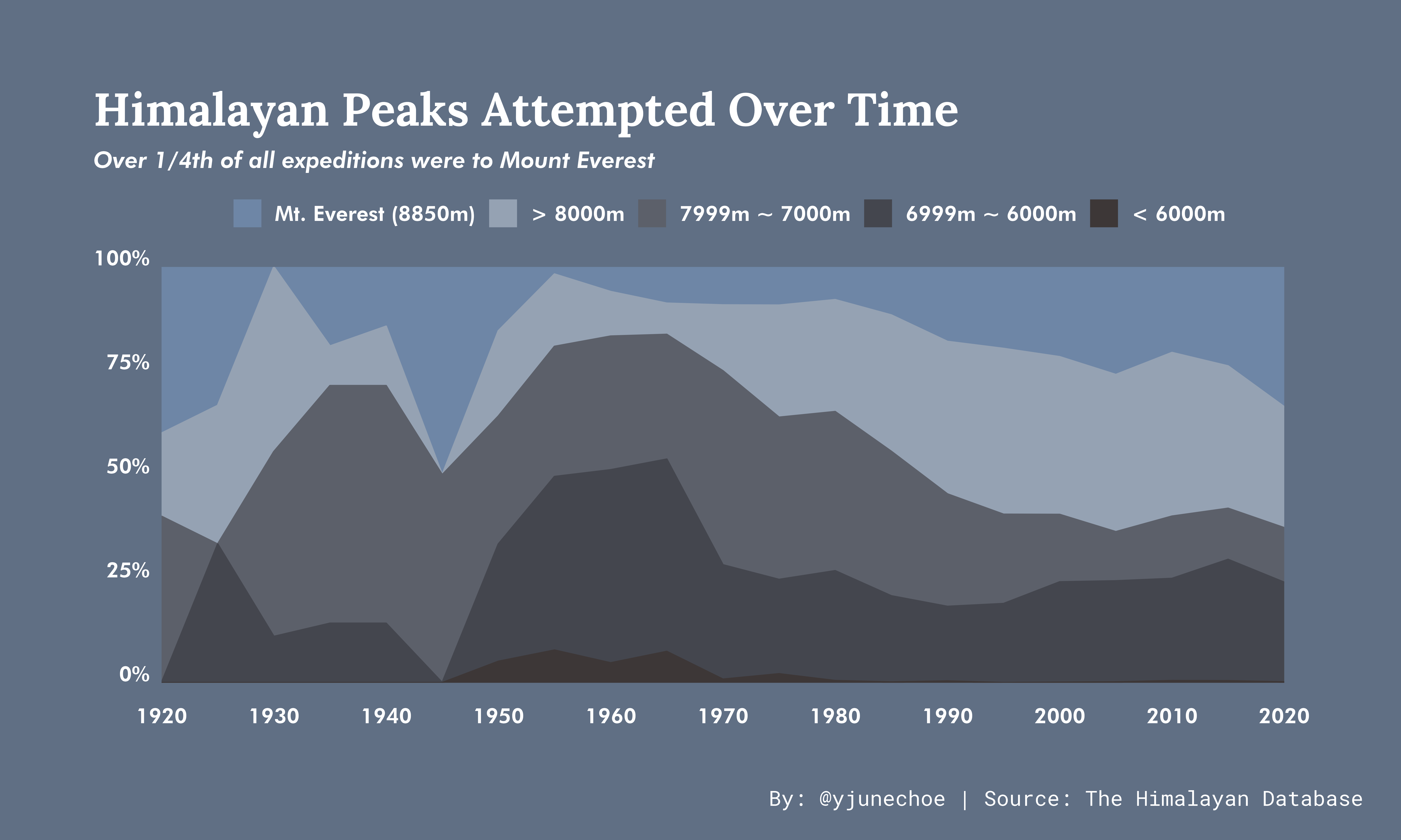
Stacked area plot of the heights of Himalayan peaks attempted over the last century

Author

Affiliation

June Choe

University of Pennsylvania Linguistics

Visualization

Things I learned

• Having a nice background color for the plot (and generally just working with color)

• Margin options of various kinds in theme()

• Using {scales}, pretty_breaks() in particular

• Using {ragg} to draw and save high quality plots

Things to improve

• The subtitle is kinda boring (and the entire plot is a bit underwhelming)

• Figure out how to increase spacing between y-axis text and the plot (hjust is relative to each label, so doesn’t work)

Code

Also available on github

library(tidyverse)

# DATA

tuesdata <- tidytuesdayR::tt_load("2020-09-22")

climb_data <- tuesdata$expeditions %>% 
  left_join(tuesdata$peaks, by = "peak_name") %>% 
  select(peak = peak_name, year, height = height_metres) %>% 
  arrange(-height) %>% 
  mutate(height_group = fct_inorder(case_when(peak == "Everest" ~ "Mt. Everest (8850m)",
                                              between(height, 8000, 8849) ~ "> 8000m",
                                              between(height, 7000, 7999) ~ "7999m ~ 7000m",
                                              between(height, 6000, 6999) ~ "6999m ~ 6000m",
                                              TRUE ~ "< 6000m"))
  ) %>% 
  count(five_years = round(year/5) * 5, height_group) %>% 
  filter(five_years >= 1920) %>% 
  complete(five_years, height_group, fill = list(n = 0)) %>% 
  group_by(five_years) %>% 
  mutate(prop = n / sum(n)) %>% 
  ungroup()


# PLOT

mountain_palette <- c("#6E86A6", "#95A2B3", "#5C606A", "#44464E", "#3D3737")

climb_plot <- climb_data %>% 
  ggplot(aes(five_years, prop)) +
  geom_area(aes(fill = height_group, color = height_group))  +
  scale_fill_manual(values = mountain_palette) +
  scale_color_manual(values = mountain_palette) +
  coord_cartesian(xlim = c(1920, 2020), expand = FALSE) +
  scale_x_continuous(breaks = scales::pretty_breaks(11)) +
  scale_y_continuous(labels = scales::percent) +
  labs(
    title = "Himalayan Peaks Attempted Over Time",
    subtitle = "Over 1/4th of all expeditions were to Mount Everest",
    x = NULL, y = NULL, fill = NULL, color = NULL,
    caption = "By: @yjunechoe | Source: The Himalayan Database"
  ) +
  theme_classic(base_family = "Futura Hv BT", base_size = 16) +
  theme(
    plot.title.position = "plot",
    plot.title = element_text(size = 28, color = "white", family = "Lora", face = "bold"),
    plot.subtitle = element_text(size = 14, color = "white", face = "italic"),
    plot.margin = margin(2, 2.5, 2, 2, 'cm'),
    plot.caption = element_text(color = "white", family = "Roboto Mono", hjust = 1.15, vjust = -13),
    legend.position = "top",
    legend.direction = "horizontal",
    legend.text = element_text(color = "white"),
    legend.background = element_rect(fill = NA),
    axis.text = element_text(color = "white"),
    axis.text.y = element_text(vjust = -.1),
    axis.text.x = element_text(vjust = -2),
    axis.ticks = element_blank(),
    axis.line = element_blank(),
    panel.background = element_blank(),
    plot.background = element_rect(fill = "#606F84", color = NA)
  )


# SAVE

pngfile <- fs::path(getwd(), "plot.png")
ragg::agg_png(
  pngfile,
  width = 60,
  height = 36,
  units = "cm",
  res = 300,
  scaling = 2
)
plot(climb_plot); invisible(dev.off())