You can inspect after_stat() and after_scale() contexts, but there’s a twist.
Motivation
The functions after_stat() and after_scale() (and the more primitive form stage()) in ggplot let you access variables that are calculated internally in the layer-building pipeline. For example:
library(ggplot2)
library(colorspace)
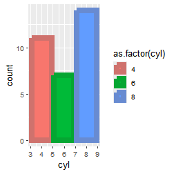
ggplot(mtcars, aes(cyl, fill = as.factor(cyl))) +
geom_bar(
aes(
y = after_stat(count),
color = after_scale(darken(fill))
),
linewidth = 3
)
We typically get limited visibility into the process. Unless…
Hacks
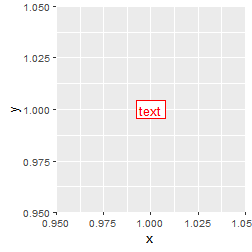
Let’s use a trivial example to mess around with:
p <- ggplot(data.frame(x = 1, y = 1), aes(x, y)) +
  geom_label()
p +
  aes(
    label = after_stat("text"),
    color = after_scale("red")
  )
We can grab variables in the data-mask with ls(.top_env) and print them:
invisible(ggplot_build(
  p +
    aes(
      label = after_stat({
        cat("after stat variables:\n")
        print(ls(.top_env))
        "text"
      }),
      color = after_scale({
        cat("\nafter scale variables:\n")
        print(ls(.top_env))
        "red"
      })
    )
))
#> after stat variables:
#> [1] "group" "PANEL" "x"     "y"
#>
#> after scale variables:
#>  [1] "alpha"      "angle"      "colour"     "family"     "fill"
#>  [6] "fontface"   "group"      "hjust"      "label"      "lineheight"
#> [11] "linetype"   "linewidth"  "nudge_x"    "nudge_y"    "PANEL"
#> [16] "size"       "vjust"      "x"          "y"
Note that this doesn’t fully reconstruct the layer data; namely, the column order is lost.
We can also print their values. Here, I’m throwing them into a dataframe to compactly display all of them
invisible(ggplot_build(
  p +
    aes(
      label = after_stat({
        cat("after stat variables:\n")
        print(as.data.frame(mget(ls(.top_env), .top_env)))
        "text"
      }),
      color = after_scale({
        cat("\nafter scale variables:\n")
        print(as.data.frame(mget(ls(.top_env), .top_env)))
        "red"
      })
    )
))
#> after stat variables:
#>   group PANEL x y
#> 1    -1     1 1 1
#>
#> after scale variables:
#>   alpha angle colour family  fill fontface group hjust label lineheight
#> 1    NA     0  black        white        1    -1   0.5  text        1.2
#>   linetype linewidth nudge_x nudge_y PANEL     size vjust x y
#> 1        1      0.25       0       0     1 3.866058   0.5 1 1
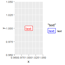
What’s funny about this is that if you add a legend to the plot, after_scale() is evaluated twice.
invisible(ggplot_build(
  p +
    aes(
      label = after_stat({
        cat("after stat variables:\n")
        print(as.data.frame(mget(ls(.top_env), .top_env)))
        "text"
      }),
      color = after_scale({
        cat("\nafter scale variables:\n")
        print(as.data.frame(mget(ls(.top_env), .top_env)))
        "red"
      })
    ) +
    scale_discrete_identity("label", guide = "legend")
))
#> after stat variables:
#>   group PANEL x y
#> 1    -1     1 1 1
#>
#> after scale variables:
#>   alpha angle colour family  fill fontface hjust label lineheight linetype
#> 1    NA     0  black        white        1   0.5  text        1.2        1
#>   linewidth     size vjust
#> 1      0.25 3.866058   0.5
#>
#> after scale variables:
#>   alpha angle colour family  fill fontface group hjust label lineheight
#> 1    NA     0  black        white        1    -1   0.5  text        1.2
#>   linetype linewidth nudge_x nudge_y PANEL     size vjust x y
#> 1        1      0.25       0       0     1 3.866058   0.5 1 1
This is a relatively new in internal change in ggplot.
That’s because after scale mappings are resolved once for the guides, and then a second time for the layer geom.
Inspect the stack
The only way to disambiguate the two after_scale() evaluations is to see where they were called from. Unfortunately, sys.calls() doesn’t seem to work.
invisible(ggplot_build(
  p +
    aes(
      label = after_stat({
        print(sys.calls())
        "text"
      }),
      color = after_scale({
        print(sys.calls())
        "red"
      })
    ) +
    scale_discrete_identity("label", guide = "legend")
))
#> NULL
#> NULL
#> NULL
For some reason, you need to wrap sys.calls() in a function to recover the stack. So I write a IIFE here:
invisible(ggplot_build(
  p +
    aes(
      label = after_stat({
        print((\()sys.calls())() |> length())
        "text"
      }),
      color = after_scale({
        print((\()sys.calls())() |> length())
        "red"
      })
    ) +
    scale_discrete_identity("label", guide = "legend")
))
#> [1] 44
#> [1] 58
#> [1] 52
Ok good. So back on after scale, if we only want to evaluate something in the after scale context for the layer (not the legend), we wanna latch onto some identifiable call upstream. I’m gonna use called-from-by_layer() as the proxy here.
called_from_by_layer <- function(x) {
  any(as.character(sapply(x, `[[`, 1)) == "by_layer")
}
So then we can use that to return different values for the layer geom vs. the legend.
p +
  aes(
    label = after_stat("text"),
    color = after_scale({
      if (called_from_by_layer((\()sys.calls())())) {
        "red"
      } else {
        "blue"
      }
    })
  ) +
  scale_discrete_identity("label", guide = "legend")
Just use ggtrace
Don’t actually do all of this though. If you’re curious about the internals, just use ggtrace! :)
sessionInfo()
Session info
sessionInfo()
#> R version 4.4.1 (2024-06-14 ucrt)
#> Platform: x86_64-w64-mingw32/x64
#> Running under: Windows 11 x64 (build 26100)
#>
#> Matrix products: default
#>
#>
#> locale:
#> [1] LC_COLLATE=English_United States.utf8
#> [2] LC_CTYPE=English_United States.utf8
#> [3] LC_MONETARY=English_United States.utf8
#> [4] LC_NUMERIC=C
#> [5] LC_TIME=English_United States.utf8
#>
#> time zone: America/New_York
#> tzcode source: internal
#>
#> attached base packages:
#> [1] stats     graphics  grDevices utils     datasets  methods   base
#>
#> other attached packages:
#> [1] colorspace_2.1-1   ggplot2_3.5.2.9001
#>
#> loaded via a namespace (and not attached):
#>  [1] vctrs_0.6.5            cli_3.6.3              rlang_1.1.4
#>  [4] xfun_0.52              generics_0.1.3         S7_0.2.0
#>  [7] litedown_0.7.1         glue_1.7.0             labeling_0.4.3
#> [10] scales_1.4.0           grid_4.4.1             tibble_3.2.1
#> [13] lifecycle_1.0.4        compiler_4.4.1         dplyr_1.1.4
#> [16] codetools_0.2-20       RColorBrewer_1.1-3     pkgconfig_2.0.3
#> [19] rstudioapi_0.17.1.9000 farver_2.1.2           R6_2.6.1
#> [22] tidyselect_1.2.1       pillar_1.10.1          commonmark_1.9.5
#> [25] magrittr_2.0.3         tools_4.4.1            withr_3.0.2
#> [28] gtable_0.3.6